Structural Elements
Introduction
An important aspect of geomechanical analysis and design is the use of structural support to stabilize a soil or rock mass. The term support describes engineered materials used to restrict displacements in the immediate vicinity of an opening. In this section, we focus on support provided to reinforce the soil or rock. 3DEC-specific support elements are described here. Other types of support may also be used by 3DEC (and FLAC3D and PFC). These are described in the following sections in the Program Guide \(\rightarrow\) Structural Elements section of the documentation.
- Beam Structural Elements
- Cable Structural Elements
- Pile Structural Elements
- Shell Structural Elements
- Geogrid Structural Elements
- Liner Structural Elements
The 3DEC-specific reinforcement types are described separately, below. In all cases, the commands necessary to define the structure(s) are quite simple, but they invoke a very powerful and flexible structural logic. This logic is developed with the same finite-difference algorithms as the rest of the code (as opposed to a matrix-solution approach), allowing the structure to accommodate large displacements, and to be applied for dynamic as well as static analysis. (See the dynamic analysis option discussed in “Dynamic Analysis.”)
Rock Reinforcement
There are several different types of reinforcement designed to operate effectively in a range of ground conditions. One type is represented by a reinforcing bar or bolt fully encapsulated in a strong, stiff resin or grout. This system is characterized by the relatively large axial resistance to extensions that can be developed over a relatively short length of the shank of the bolt, and by the high resistance to shear that can be developed by an element penetrating a slipping joint. A second type of reinforcement system, represented by cement-grouted cables or tendons, offers little resistance to joint shear, and development of full axial load may require deformation of the grout over a substantial length of the reinforcing element. These two types of reinforcement are identified, respectively, as local reinforcement and global (or spatially extensive) reinforcement. The characteristic behavior of these two rock reinforcement systems has been incorporated into 3DEC.
Local Reinforcement at Joints (sel reinforcement command)
The local reinforcement formulation considers only the local effect of reinforcement where it passes through existing discontinuities. The formulation results from observations of laboratory tests of fully grouted untensioned reinforcement in good quality rocks with one discontinuity, which indicate that strains in the reinforcement are concentrated across the discontinuity (Bjurstrom 1974 and Pells 1974). This behavior can be achieved in the computational model by calculating, for each element, the forces generated by displacements across the discontinuity through which the element passes. The following description of this formulation is taken from Lorig (1985).
This formulation exploits simple force-displacement relations to describe both the shear and axial behavior of reinforcement across discontinuities. Large shear displacements are accommodated by considering the simple geometric changes that develop locally in the reinforcement near a discontinuity. Although the local reinforcement model can be used with either rigid blocks or deformable blocks, the representation is most applicable to cases in which deformation of individual rock blocks may be neglected in comparison with deformation of the reinforcing system. In such cases, attention may be focused reasonably on the effect of reinforcement near discontinuities.
Axial Behavior
Historically, axial testing of rock reinforcement has focused on pull-out tests for two reasons:
- ease of experimentation and interpretation of results; and
- provision of axial restraint (the main function of reinforcement in the prevailing conceptual models).
Consequently, a relatively good understanding of axial force-displacement relations has been achieved. The axial force-displacement relation typically used in the representation of rock reinforcement is shown in Figure 1.
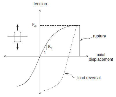
Figure 1: Axial behavior of local reinforcement systems.
Figure 1 indicates an identical response in tension and compression. This may not be the case for all reinforcing systems.
If pull-test results are not available, the following theoretical expression (given by Gerdeen et al. 1977) may be used to estimate the axial stiffness, \(K_a\), for fully bonded solid reinforcing elements:
where:
\(d\)1 = reinforcement diameter;
\(k\) = \([{{1} \over {2}}\ G_g\ E_b\ /\ (d_2\ /\ d_1 - 1)]^{1/2}\)
\(G_g\) = grout shear modulus;
\(E_b\) = Young’s modulus of reinforcement material; and
\(d\)2 = hole diameter.
Comparisons with finite element analyses (Gerdeen et al. 1977) indicate that Equation (1) tends to slightly overestimate axial stiffnesses.
The ultimate axial capacity of the reinforcement depends on a number of factors, including strength of the reinforcing element, bond strength, hole roughness, grout strength, rock strength, and hole diameter. In the absence of results of physical tests, empirical relations may be used to estimate the ultimate anchorage strength, \(P_{ult}\). One such relation for the design of cement-grouted reinforcement is given by Littlejohn and Bruce (1975):
where:
\(\sigma_c\) = uniaxial compressive strength of massive rocks (100% core recovery) up to a maximum value of 42 MPa, assuming that the compressive strength of the cement grout is equal to or greater than 42 MPa; and
\(L\) = bond length.
Shear Behavior
Recognition that reinforcement also acts to modify the shear stiffness and strength of discontinuities has led to laboratory shear testing of reinforced discontinuities. Experimental results and theoretical investigations indicate that shearing along a discontinuity induces bending stresses in the reinforcement that decay very rapidly with distance into the rock from the shear surface. Typically, the bending stresses are insignificant within one to two reinforcing element diameters.
The shear force-displacement relation typically used to represent shear behavior is shown in Figure 2. The figure shows representative responses for reinforcement at various altitudes with respect to the traversed discontinuity and direction of shear.
If the results of physical tests are not available, the shear stiffness, \(K_s\), may be estimated using the following expression from Gerdeen et al. (1977):
where:
\(\beta\) = \([K\ /\ (4\ E_b\ I)]^{1/4}\);
\(K\) = \(2E_g\ /\ (d_2/d_1 - 1)\);
\(I\) = second moment of area of the reinforcement element; and
\(E_g\) = Young’s modulus of the grout.
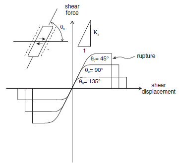
Figure 2: Shear behavior of reinforcement system.
Empirical relations can be used to estimate the maximum shear force, \(F_{s,b}^{max}\), for a reinforcement element at various orientations with respect to a transgressed discontinuity and direction of shear. For example, Bjurstrom (1974) used the results of shear tests of ungrouted reinforcement perpendicular to a discontinuity in granite to develop the expression
where \(\sigma_b\) = yield strength of reinforcement.
In their assessment of maximum shear resistance, St. John and Van Dillen (1983) applied the results of Azuar et al. (1979). The latter found that the maximum shear force was about half the product of the uniaxial tensile strength of the reinforcement and its cross-sectional area for reinforcement perpendicular to the discontinuity. The force increased to 80-90% of that product for reinforcement inclined with the direction of shear. Shear displacements causing rupture were reported after approximately two reinforcement diameters for the perpendicular case, and one diameter for the inclined case. St. John and Van Dillen interpreted differences between strength and amount of displacement before rupture in terms of the extent of crushing of rock around the reinforcement.
Numerical Formulation
The model in 3DEC assumes that, during shear displacement along a discontinuity, the reinforcement deforms as shown in Figure #the-sel3-cfyt. The short length of reinforcement that spans the discontinuity and changes orientation during shear displacement is referred to as the active length. The assumed geometric changes were originally suggested in a derivation by Haas (1976) for conventional point-anchored reinforcement, and adopted by Fuller and Cox (1978) in considering fully grouted reinforcement.
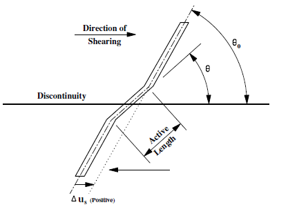
Figure 3: Assumed reinforcement geometry after shear displacement, \(\Delta u_s\).
It is assumed that the active length changes orientation only as a direct geometric result of shear and normal displacements at the discontinuity. Methods for estimating the active length are presented in the next section. The model may be considered to consist of two springs located at the discontinuity interface and oriented parallel and perpendicular to the reinforcement axis, as shown in Figure 4. Following shear displacement, the axial spring is oriented parallel to the active length, while the shear spring remains perpendicular to the original orientation, as shown in Figure 4. Similar geometric changes follow displacements normal to the discontinuity.
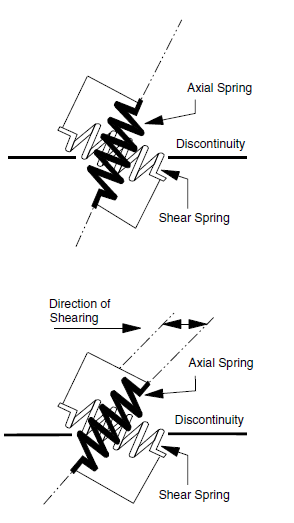
Figure 4: Orientation of shear and axial springs representing reinforcement prior to and after shear displacement.
The force-displacement models used in 3DEC to represent axial and shear behavior are continuous linear algorithms written in terms of stiffness (axial or shear) and the ultimate load capacity. Note that the formulation for local reinforcement in 3DEC is a simplified version of the general formulation implemented in UDEC (see Itasca 2011).
The force-displacement relation that describes the axial response is given by
where:
\(\Delta F_a\) is an incremental change in axial force;
\(\Delta u_a\) is an incremental change in axial displacement; and
\(K_a\) is the axial stiffness.
In this formulation, no reduction in stiffness is made to account for crushing of the grout and/or rock near the discontinuity.
A rupture limit can be specified for the axial force. If the extensional axial strain in the reinforcement element exceeds a specified strain limit, then the axial force will be set to zero.
The shear force-displacement relation is described in incremental form by the expression
where:
\(\Delta F_s\) is an incremental change in shear force;
\(\Delta u_s\) is an incremental change in shear displacement; and
\(K_s\) is the shear stiffness.
A rupture limit can also be specified for the shear force. If the relative shear strain in the reinforcement element exceeds a specified strain limit, then the shear force will be set to zero.
The force-displacement relations described above are used to determine forces in the springs arising from incremental displacements at the endpoints of the active length. The resultant shear and axial forces are resolved into components parallel and perpendicular to the discontinuity, as shown in Figure 5. Forces are then applied to the neighboring blocks.
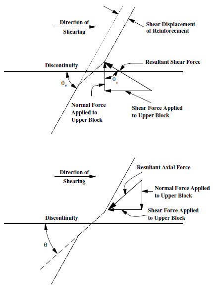
Figure 5: Resolution of reinforcement shear and axial forces into components parallel and perpendicular to discontinuity.
Estimation of Active Length
To define the assumed local deformation illustrated in Figure 3, an estimate of the active length is required. It has been shown that the active length extends approximately one to two reinforcing element diameters on either side of the discontinuity. In the absence of experimental data, results of theoretical analysis may be used to define the active length. For example, in defining the elastic shear stiffness, \(K_s\), Gerdeen et al. (1977) also determine a quantity, l, called the load transfer length, or “decay length.” If \(\rho_{max}\) is the proportion of maximum deflection in the reinforcement, the relation between it and the load transfer length may be expressed by
For example, the point at which the deflection decays to 5% of its maximum value is
or
This approach was developed for reinforcement oriented perpendicular to the shear plane. Dight (1982) presents a theoretical analysis for determining the distance from the shear plane to maximum moment which corresponds with the location of the plastic hinge in the reinforcement element. This approach places no restrictions on the orientation of the reinforcement with respect to the shear plane. A significant result of this analysis is that the distance of the plastic hinge from the shear plane does not appear to vary greatly with shear displacement, especially for displacements greater than 10 mm (0.4 in) for typical reinforcement systems. This observation is in agreement with the assumed geometry changes described earlier.
Local Reinforcement Properties
The local reinforcement elements used in 3DEC require the following input parameters:
stiffness-axial: axial stiffness [force/length];yield-tension-force: ultimate axial capacity [force];rupture-axial-strain: extensional failure strain (default = infinite) [ – ];stiffness-shear: shear stiffness [force/length];yield-shear-force: ultimate shear capacity [force];rupture-shear-strain: shear failure strain (default = infinite) [ – ];active-half-length: 1/2 active length [length];
The axial stiffness and ultimate axial capacity are usually determined to best-fit pull-out tests as described in the Axial Behavior section. The axial force-displacement relation follows a constant axial stiffness until the ultimate axial capacity is reached.
The value for 1/2 the active length can also be back-calculated from experimental testing, as discussed in the sections Shear Behavior and Estimation of Active Length.
Summary of Commands Associated with Local Reinforcement Elements
All of the commands associated with local reinforcement elements are listed in Table 1. See Commands for a detailed explanation of these commands.
sel reinforcement create |
sel reinforcement group |
sel reinforcement history |
sel reinforcement list |
sel reinforcement property |
Example Application — Reinforced Slope
The stability analysis of the rock slope described in the tutorial in Tutorial: Quick Start is repeated using the local reinforcement elements to represent rock anchors. The slope is stabilized by adding two horizontal lines of local reinforcement. One line extends from location (30,40,25) to location (70,40,25), and the other from location (30,20,25) to location (70,20,25). When the joint friction is reduced, the slope is then stable, as indicated by Figure 6. A history of y-displacement at a point on the slope face also shows that motion is restrained by the reinforcement (see Figure 7). The input commands for this example are listed in Example reinforcement.dat.
reinforcement.dat
model new
model large-strain on
model title 'ROCK SLOPE STABILITY --- WEDGE STABLE WITH LOCAL REINFORCEMENT'

block create brick 0,80 -30,80 0,50
block group "rock"

; boundary blocks on sides of slope
block cut joint-set dip 90 dip-direction 180 ori 0,0,0
block cut joint-set dip 90 dip-direction 180 ori 0,50,0
block hide range pos-x 0,80 pos-y -30,0 pos-z 0,50
block hide range pos-x 0,80 pos-y 50,80 pos-z 0,50
block group  "slope rock"

; shallow-dipping fracture planes
block cut joint-set dip 2.45 dip-direction 235 ori 30,0,12.5
block cut joint-set dip 2.45 dip-direction 315 ori 35,0,30

; high angle foliation planes
block cut joint-set dip 76 dip-direction 270 spac 4 num 5 ori 38,0,12.5
block hide range pos-x 30,80  pos-y 0,50 pos-z 0,50
block cut joint-set dip 0 dip-direction 0 ori 0,0,10
block hide range pos-x 0,80 pos-y -30,80 pos-z 0,10
block group "excavation"
block hide off

block hide range group "rock"
block hide range pos-x  0,80 pos-y 0,50 pos-z 0,10
block hide range pos-x 55,80 pos-y 0,50 pos-z 0,50
block hide range pos-x  0,30 pos-y 0,50 pos-z 0,50

; intersecting discontinuities
block cut joint-set dip 70 dip-direction 200 ori 0,35,0
block cut joint-set dip 60 dip-direction 330 ori 50,15,50
block hide off

; fix boundary blocks and initialize gravity
block fix range pos-x  0,80 pos-y 0,50 pos-z 0,10
block fix range pos-x 55,80 pos-y 0,50 pos-z 0,50
block fix range group "rock"

block delete range group "excavation"

model gravity 0 0 -10
;
; assign properties
block property density 2000

block contact generate-subcontacts
; 0 friction between boundary blocks and slope blocks
block contact property stiffness-normal 1e9 stiffness-shear 1e9 friction 0

; set high friction in slope blocks for now
block hide range group "rock"
block contact property friction 89
block contact material-table default prop stiffness-normal 1e9 ...
                                          stiffness-shear 1e9 fric 6.0

; set up history on potential wedge
block hide range plane dip 70 dip-dir 200 or 0,35,0 below
block history disp-z position 30 30 30
block hide off
block hide range group "rock"
model solve
model save 'slope'

; add local reinforcement
sel reinforcement create by-line (30 25 40) (70 25 40) property 1
sel reinforcement create by-line (30 25 20) (70 25 20) property 1
sel reinforcement property 1 stiffness-axial 1e8 ...
                             active-half-length 1.0 yield-tension-force 1e8

block contact property friction 6.0 ;range group-int "slope rock" "slope rock"

history purge
block gridpoint initialize displacement 0 0 0
model cycle 5000

model save 'slope_st'
program return
Figure 6: Stabilization of slope by reinforcement.
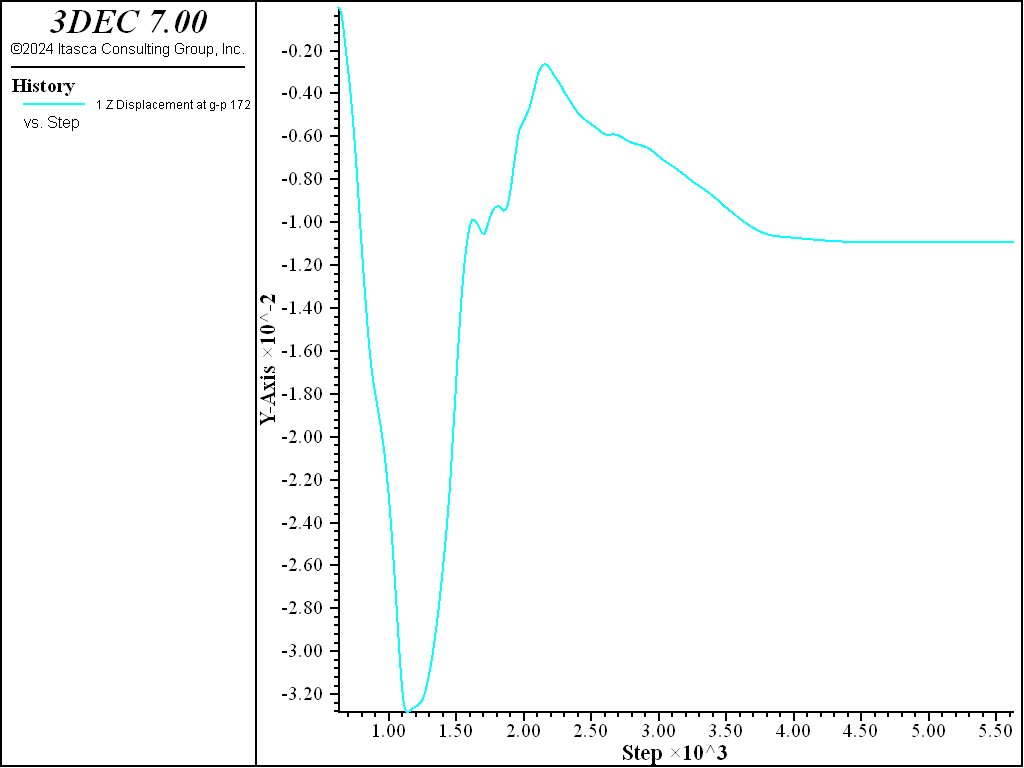
Figure 7: z-displacement history at (30, 30, 30) on slope face.
Hybrid Bolts (sel hybrid command)
In assessing the support provided by rock reinforcement, it is often necessary to consider not only the local restraint provided by reinforcement where it crosses discontinuities, but also the restraint to intact rock that may experience inelastic deformation in the failed region surrounding an excavation. Such situations arise in modeling inelastic deformations associated with failed rock and/or reinforcement systems (e.g., cable bolts) in which the bonding agent (grout) may fail in shear over some length of the reinforcement.
Cable elements in 3DEC (Cable Structural Elements) allow the modeling of a shearing resistance along their length, as provided by the shear resistance (bond) between the grout and either the cable or the host medium. The cable is assumed to be divided into a number of segments of length, \(L\), with nodal points located at each segment end. The mass of each segment is lumped at the nodal points, as shown in Figure 8. Shearing resistance is represented by spring/slider connections between the structural nodes and the block zones in which the nodes are located.
To use the cable logic, deformable blocks must be specified, and the blocks must be made deformable before the cable elements are installed. Each structural node is associated with a finite volume zone for calculation of shear forces between the cable and the zones.
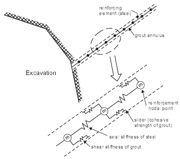
Figure 8: Conceptual mechanical representation of fully bonded reinforcement, which accounts for shear behavior of the grout annulus.
A full description of the cable behavior is given in Cable Structural Elements section.
Basic cable elements do not resist shearing perpendicular to the cable. However, when cables are used to simulate bolts, it is well known that bolts crossing joints will provide some resistance to shearing on the joints. Dight (1982) suggests five different mechanisms that contribute to this effect.
- An increase in shear resistance due to lateral resistance developed by the rockbolt via dowel action
- An increase in normal stress as a result of pre-stressing of the rockbolt
- An increase in normal stress as a result of axial force developed in the rockbolt from dilatancy of the joint
- An increase in normal stress as a result of axial force developed in the rockbolt from lateral extension
- An increase in shear resistance due to axial force in the rockbolt resolved in the direction of the joint
Cables in 3DEC will demonstrate effects 2 – 5, but not 1. The dowel action is really an umbrella term for a set of complex mechanical effects including bending of the steel bolt, crushing of the grout, crushing of the host rock, etc. (see Figure 9). No attempt is made to reproduce all of these effects in 3DEC. Instead, the dowel effect is simulated simply by a shear spring that resists slip on the fault where it is crossed by the bolt. The hybrid bolt is therefore a combination of cable element and reinforcement element.
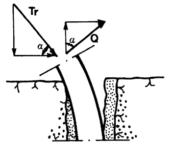
Figure 9: Resistance mechanism of a rock joint reinforced by means of a dowel (from Ferrero, 1995).
The formulation of the cable portion is exactly as described in Cable Structural Elements. The formulation for the dowel is almost exactly the same as that for local reinforcements (Local Reinforcement). The following differences should be noted.
- There is no axial component to the dowel spring. This is because it is assumed that the cable itself will provide axial forces.
- The shear spring is always oriented parallel to the joint, regardless of the cable orientation relative to the joint. This is to avoid spurious axial components of force.
- When the dowel ruptures (the shear strain limit is surpassed), the host cable also ruptures at the same location.
- Shear strength may be orientation-dependent (see below).
The dowel shear force-displacement relation is described in incremental form by Equation (6). A yield strength can be specified for the shear force. This shear yield strength may be orientation-dependent (see below). When the yield strength is exceeded, the dowel behaves plastically and the shear resistance remains constant as shear displacement continues. A rupture limit (strain) may also be specified. If the relative shear strain in the reinforcement element exceeds a specified strain limit, then the shear force will be set to zero. As mentioned above, the host cable will also rupture and its axial force will be set to 0.
The shear forces are applied to the faces of the blocks on either side of the joint by interpolating to the zone face nodes. The dowel formulation only works with deformable (zoned) blocks.
Geometry
By default, the hybrid bolt segment lengths are constant. With the sel hybrid create command, the user can specify either segments for the number of segments, or segment-length for the approximate segment length. If segment-length is used, the resulting segment length may be slightly different than specified to ensure an integer number of segments of equal length.
The dowel-length parameter is the length of the dowel segment. The length of the dowel segment is only used in the calculation of shear strain (= shear displacement / dowel-length). It has no effect on the calculated forces or on the node placement. See Figure 10.
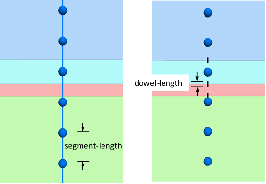
Figure 10: A hybrid bolt passing across three joints. The cable segments and nodes are shown in the left plot. Nodes and dowels (black lines) are shown in the right plot.
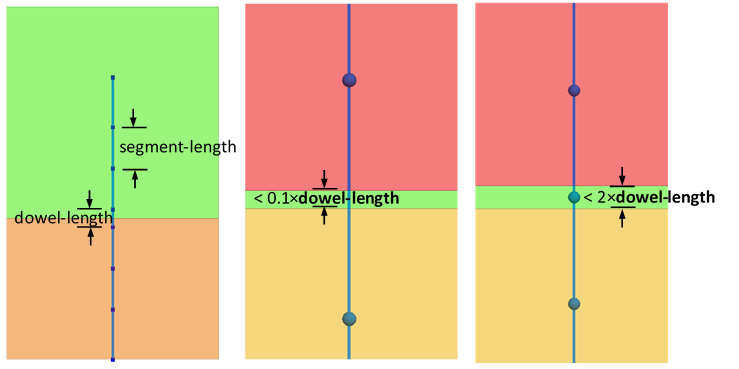
It is recognized that the distribution of nodes around faults has an effect on the bolt behavior. It is possible to create a hybrid bolt and ensure that there is at least one node within each block (between each pair of joints). This is done when evoking the hybrid create command with the keyword spacing variable.
In this mode, the keyword segment-length dictates the length of cable bolt segments inside blocks (between joints) and dowel-length gives the length of bolt elements that cross joints. If dowel-length is not given, then it defaults to segment-length. An example is shown in Figure 11. If a block is smaller than 0.1 × dowel-length, no node is placed in the block. If a block is larger than 0.1 × dowel-length but smaller than 2 × dowel-length, then a single node is placed in the middle of the block.
The dowel-length parameter is also the length of the dowel segment used in the calculation of shear strain (=shear displacement / dowel-length).
Warning
With spacing variable, it is possible to create a bolt with very short cable segments if joints are close together. These short segments have a tendency to rupture at low stress since the axial strain can grow large for small amounts of displacement. If this is a concern the default (spacing constant) should be used.
In general, the node spacing used for the calibration should be equal to the one used in the real problem in 3DEC. In particular, dowel-length should be chosen small compared to the block size, so that it remains constant as much as possible across the model. Indeed, if the specified segment-length/dowel-length is too big compared to the block size, it will get automatically reduced by 3DEC (if using spacing variable) or the bolt might miss the impact of certain closely spaced joints (if using spacing constant) and the calibrated behavior will significantly differ from the bolt behavior in the large-scale model.
Hybrid Bolt Properties
There are 11 properties associated with the cable portion of the hybrid bolt. Advice on choosing these parameters is given in the section i Cable Properties.
density, mass density, \(ρ\) (optional — needed if dynamic mode or gravity is active) [M/L3]young, Young’s modulus, \(E\) [F/L2]grout-cohesion, grout cohesive strength (force) per unit length, \(c_g\) [F/L]grout-friction, grout friction angle, \(\phi_g\) [degrees]grout-stiffness, grout stiffness per unit length, \(k_g\) [F/L2]perimeter, grout exposed perimeter, \(p_g\) [L]thermal-expansion, thermal-expansion coefficient, \(\alpha_t\) [1/T] (optional — used for thermal analysis)cross-sectional-area, cross-sectional area, \(A\) [L2]yield-compression, compressive yield strength (force), \(F_c\) [F]yield-tension, tensile yield strength (force), \(F_t\) [F]rupture-tension-strain, tensile strain limit, [-]
Hybrid bolts have three extra properties associated with the dowel segments:
dowel-stiffness, shear stiffness of the dowel, [F/L]dowel-yield, dowel shear force yield limit, [F]dowel-strainlimit, dowel shear strain limit, [-]
These properties are generally chosen by calibrating against laboratory shear tests. An easy-to-use HTML Calibration Tool is accessible from this documentation (see below).
Calibration
Influence of Segment Length and Dowel Length
For a fixed set of parameters, changing the node spacing mostly influences the rupture displacement in axial and shear — easy to readjust by changing the axial and shear critical strain — but also the stiffness of the bolt. Indeed, for a given shear or axial joint displacement/opening, the smaller the node spacing, the stiffer the bolt reaction will be due to an increase in component (4) described above (increase in normal stress as a result of axial force developed in the rockbolt from lateral extension). One can adjust the shear and axial stiffness then, but there is a limitation to the calibration process: the smaller the segment, the larger the influence of the axial stiffness on the shear response of the bolt. Indeed, the smaller the node spacing, the larger the axial strain becomes for a given joint shear displacement relative to the shear strain. This is a geometric effect that the calibration can not overcome if segment-length is fixed to dowel-length.
Overall, it is important to realize that the micro-axial behavior strongly influences the macro-shear behavior of the bolt.
The Calibration Steps
The hybrid bolt model properties are typically calibrated through simple shear and pullout tests on bolts perpendicular to the joint (see example below).
Table 2 presents the parameters that should be defined before performing the calibration and held constant during a simulation for the calibration to remain valid.
| 3DEC Parameter | Description | Depends on |
|---|---|---|
cross-sectional-area |
Cross-sectional area of cable | Support design |
perimeter |
Perimeter of the hole. Only required if grout-friction > 0 |
Borehole diameter |
segment-length |
Hybrid bolt node spacing inside blocks | Geometry of the model and especially of the blocks used to model the rock mass. segment-length should be small enough to have at least one or two nodes in the majority of the blocks |
dowel-length |
Length of dowel segments in a hybrid bolt. Default = segment-length. The minimum hybrid bolt segment length is also calculated from this value if using spacing variable (dowel-length/10) |
Same as segment-length |
grout-friction |
Optional parameter. Friction angle of the grout material [degrees] | Grout properties |
Figure 3 presents typical simple shear test results and associated stages. Simple shear tests are the classical tests used to study (and in this case calibrate) bolt behavior in shear.
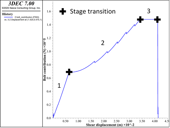
Figure 12: Hybrid bolt calibration. Typical simple shear test curve and associated stages.
Table 3 presents the critical parameters to adjust in order to obtain the desired behavior for hybrid bolts during a simple shear test.
| Stage | Primary Influence | Secondary Influence |
|---|---|---|
| Elastic stage (1) | dowel-stiffness |
young grout-stiffness |
| End of elastic stage | dowel-yield |
|
| Yield stage (2) | grout-stiffness |
young |
| End of yield stage/Plastic stage (3) | grout-cohesion |
yield-tension |
| End of plastic stage | dowel-strainlimit |
Figure 4 presents typical simple shear test results and associated stages. Pull tests are the classical tests used to study, and in this case calibrate, bolt behavior in tension.
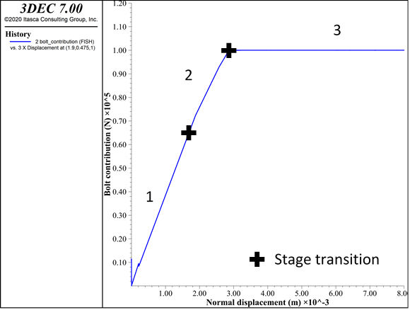
Figure 13: Hybrid bolt calibration. Typical pull test curves and associated stages.
Table 4 presents the critical parameters to adjust in order to obtain the desired behavior for hybrid bolts during a simple pull test.
| Stage | Primary Influence | Secondary Influence |
|---|---|---|
| Elastic stage (1) | young grout-stiffness |
|
| End of elastic stage | grout-cohesion |
|
| Yield stage (2) | grout-cohesion |
young |
| End of yield stage/Plastic stage (3) | yield-tension or grout-cohesion |
|
| End of plastic stage | dowel-strainlimit |
Below are a few comments to keep in mind while calibrating the hybrid bolt.
- Make sure the number of nodes and length of the cable is large enough that it does not influence the results of the calibration (i.e., ensure that the bolt length is long enough to fully exercise the bolt capacity and not get slip along the whole length of the bolt before reaching that stage).
- If the cable strain limit is very low compared to the dowel’s, then the rupture (axial and shear) will always be induced by cable (axial) rupture.
- The node spacing strongly influences the behavior of the bolt for a given joint displacement. The node spacing used for the calibration should be equal to the one used in the real problem in 3DEC. In particular, the dowel length should be chosen small compared to the block size, so that it remains constant as much as possible across the model. Indeed, if the specified
segment-length/dowel-lengthis too big compared to the block size, it will get automatically reduced by 3DEC (ifspacing=variable) or the bolt might miss the impact of certain closely spaced joints (spacing=constant) and the calibrated behavior will significantly differ from the bolt’s behavior in the large-scale model.
Orientation-Dependent Shear Strength
In the field, rock bolts can be subjected to a combination and/or succession of shear and axial solicitation in various directions. Only a few references study the effect of bolt inclination on the bolt behavior when crossing a joint. The hybrid bolt model has not been implemented to reproduce all the complexity of rock bolt behavior in every possible condition. It is built to take into account the shear resistance generated by the bolt at joint intersections in a simple manner, while accurately reproducing the support brought to the rock mass observed experimentally. This section discusses the inclination effect on a simple shear test in 3dec| for a given set of parameters and compares it to observations available in the literature.
Laboratory tests suggest the following.
- The maximum shear strength of the bolted joint increases with the joint friction angle.
- For a given joint friction angle, the maximum shear strength of the bolted joint varies with the bolt inclination.
- Inclined bolts react in a stiffer way than normal ones.
- The greatest ultimate displacement is reached when the bolt is normal to the joint.
- For very low values of friction angle, the bolt inclination has no influence on the maximum resistance.
- The confining effect increases with inclination while the cohesion term decreases.
Figure 5 shows simple shear test results for a friction angle of 40º and various bolt inclinations (from 10º to 130º).
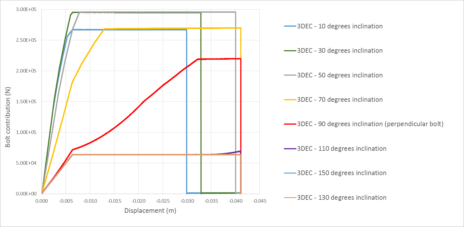
Figure 14: Bolt inclination effect on a simple shear test with a joint friction angle of 40º (inclination > 90º corresponds to bolt inclined in the opposite direction to the shearing direction).
Figure 6 shows simple pull test results for two inclination angles (from 70º to 90º).
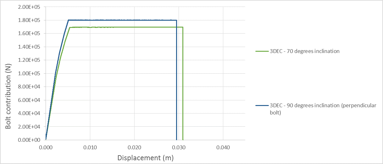
Figure 15: Bolt inclination effect on a pullout test.
Like the rock bolt behavior observed experimentally, the 3DEC hybrid bolt behaves as follows.
- Inclined bolts react in a stiffer way than normal ones. This is due to a geometrical effect. Indeed, the more the bolt is inclined (compared to the perpendicular direction to the joint), the bigger the increment of axial force in the cable for a given increment of shear displacement.
- As the bolt rotates from the perpendicular direction, the confining effect (friction effect) increases while the cohesion term (dowel action and shear cable action) decreases.
- The ultimate shear displacement leading to bolt failure varies with bolt inclination. The ultimate shear displacement is maximum when the bolt is perpendicular to the joint. In this case, it is directly related to the input dowel shear rupture strain (maximum shear displacement = maximum dowel strain × dowel length). When the bolt is more inclined (\(\theta\) > 70 degrees in Figure 5), the cable strain limit for axial rupture is reached before the dowel strain limit since the cable element gets elongated more quickly. And the more the bolt is inclined, the less joint shear displacement is necessary for the cable to reach the axial strain limit.
Note that the inclination at which the rupture strain switches from being controlled by the dowel shear limit to being controlled by the cable axial limit depends on the input values. If the cable strain limit is very low compared to the dowel’s, then the rupture will always be induced by cable (axial) rupture. If the cable strain limit is infinite, then the controlling strain limit is always the dowel (shear) strain limit, independent of the orientation.
Shear tests have also been performed on bolts inclined in the opposite direction to shearing (inclination > 90° in Figure 5). In those cases, while the joint is sheared, the cable element gets compressed (and not stretched) so that the only force applied by the bolt on the joints comes from the dowel element. At the end of the elastic stage, when the dowel reaches its yield value, the force no longer increases except if the cable element rotates enough so that it gets stretched again (this is the case at the end of the test for \(\theta\) = 110°).
Figure 6 presents pullout test results for a bolt perpendicular to the joint and one slightly inclined (\(\theta\) = 70°). When the bolt is inclined, a given increment of displacement (when the block is pulled) induces a smaller stretch than when the bolt is perpendicular to the joint. That is why the stiffness is slightly lower. This is the same geometrical effect that causes the maximum axial displacement to be higher for the inclined bolt (~31 mm) than for the perpendicular bolt (~29 mm). When the bolt is perpendicular to the joint (and so parallel to the pulling direction), the maximum load equals the cable yield capacity (18 tonnes in this case). When the bolt is inclined, the maximum load equals the projection of this value on the pulling direction. The more inclined the bolt, the lower the maximum load when compared to the yield capacity of the bolt.
Very few experimental results are available that consider an inclined bolt subjected to shearing. In terms of qualitative behavior, the 3DEC hybrid bolt reproduces most effects due to inclination described in the literature for analytical or experimental results. In terms of quantitative results, we believe the hybrid bolt behavior is reasonable considering the level of accuracy it is meant to achieve and in the order of magnitude observed in the few available experimental tests.
Effect of Joint Friction Angle on Bolt Load Capacity
During a simple shear test the three forces contributing to the bolt effect on the joint are the dowel element shear resistance (Fd), the cable shear resistance (FcS), and the additional friction force due to the cable normal force (FcN). If we consider a bolt inclination of \(\theta_1\) (so that 90º corresponds to a bolt perpendicular to the joint) and a joint friction angle of \(\phi\) degrees, the theoretical maximum bolt contribution equals:
where:
\(F_c\) = Axial force acting in the cable element whose maximum value is the input cable yield value;
\(F_d\) = Force acting in the dowel element whose maximum value is the input dowel yield value
The first term represents the shear resistance (FcS) and the second term represents the normal component (FcN).
As a consequence, the hybrid bolt contribution in 3DEC depends on the friction angle and the bolt inclination. Considering that the bolt rotates a few degrees during the simple shear test, Figure 7 gives an estimation of the three forces generated by the presence of the hybrid bolt for various bolt inclinations and for different friction angles.
Like the rock bolt behavior observed experimentally, the 3DEC hybrid bolt behaves as follows.
- For a given joint friction angle, the maximum shear strength of the bolted joint varies with the bolt inclination. For a 40 degree friction angle, the maximum value is observed around 45 degrees and corresponds to a 30% increase compared to a perpendicular bolt.
- The maximum shear strength of the bolted joint varies with the joint friction angle; the higher the friction, the higher the maximum shear strength.
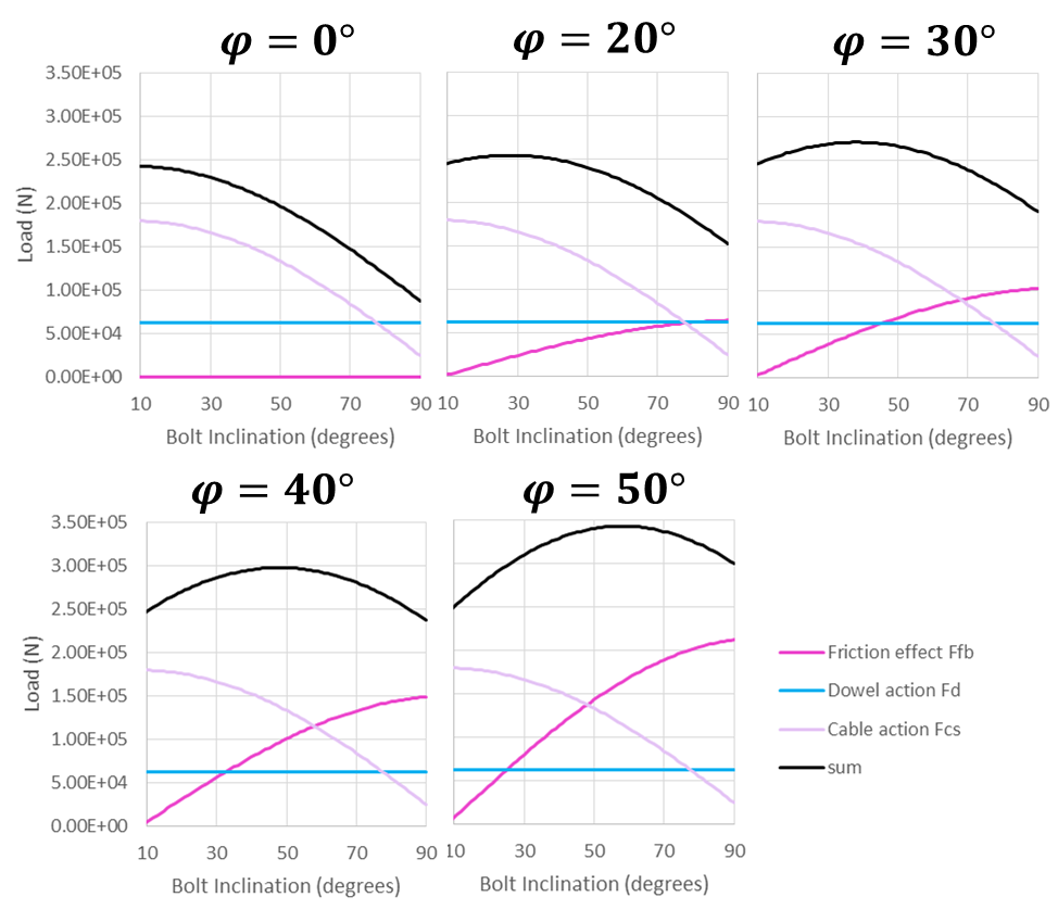
Figure 16: Variation of bolt action contributions with bolt inclination for five different joint friction angles (0º, 20º, 30º, 40º, and 50º) – a bolt inclination of 90º corresponds to a bolt perpendicular to the joint.
HTML Calibration Tool
A calibration tool for hybrid bolts is provided with this documentation to make it easier to choose bolt properties based on laboratory data. Default properties for different bolt types are also included with the tool. The tool provides its own documentation (see the “?” where it appears in the tool).
Summary of Commands Associated with Hybrid Bolts
All of the commands associated with hybrid bolts are listed in Table 5. See Commands for a detailed explanation of these commands.
sel hybrid change |
||
sel hybrid create |
||
sel hybrid delete |
||
sel hybrid group |
||
sel hybrid history |
||
sel hybrid list |
||
sel hybrid node |
||
sel hybrid property |
||
sel hybrid update |
Example Application: Simple Shear Test
A simple shear test is simulated using two blocks (Figure 17). The bottom of the left block is prevented from moving in the vertical direction and the top of the right block is moved downwards at a constant velocity. A hybrid bolt spans the joint from left to right. A normal stress of 1 MPa is applied. The friction angle of the joint is set to 40º and the cohesion is 0.
For the hybrid bolt, the dowel segment is assigned a yield strength of 0.063 MN and a strain limit of 0.41. Figure 18 shows the bolt contribution versus shear displacement. The bolt contribution is essentially the shear stress minus the frictional strength (\(\sigma_n \tan \phi\)). At about 7 mm of shear displacement, the dowel segment yields. At about 3.5 cm, the cable itself yields in tension. Finally after about 4.1 cm of shear, the dowel ruptures and the bolt fails.
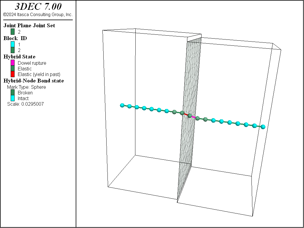
Figure 17: Blocks and bolt configuration in the shear test. Model is shown after bolt rupture.
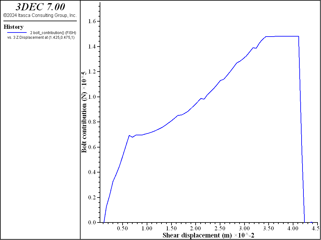
Figure 18: Bolt contribution in the shear test.
blocks.dat
;
;Build model for hybrid bolt calibration
;
model new
fish automatic-create off
model random 10000
model large-strain on
;
fish define params

  ; block dimensions
  global block_lenH = 0.95
  global block_lenV = 2.0
  global edge_length_=0.125 ; zone size

  ; block properties
  global ymod_=40e9
  global pratio_=0.25
  global dens_=2500

  ; joint properties
  global jkn_=3e11
  global jks_=3e11
  global jfric_=40.0

  ;hybrid bolt parameters
  global area_=201e-6
  global e_=1.4e11
  global grout_stiff_=3e8
  global grout_strength_=2e5
  global cable_yield_=100e3
  global cable_strain_limit_=0.2  ; tensile
  global dowel_stiffness_=1.0e7
  global dowel_yield_=62.8e3
  global dowel_strain_limit_=0.41 ; shear
  global dowel_length_=0.1
  global segment_length_=0.1

  ; calculated parameters
  global bolt_len=block_lenH*2.
end
[params]

=====================================================

;
;make 2 blocks
block create brick 0 [block_lenH] 0 [block_lenH] 0 [block_lenV]
block create brick [block_lenH] [2*block_lenH] 0 [block_lenH] 0 [block_lenV]
block zone generate edgelength [edge_length_]

; zone and contact properties
block zone cmodel elastic
block zone property young [ymod_] poisson [pratio_] density [dens_]

block contact jmodel assign mohr
block contact property stiffness-normal [jkn_] ...
                       stiffness-shear [jks_]  ...
                       friction [jfric_]
block contact mat-table default prop stiffness-normal [jkn_] ...
                                     stiffness-shear [jks_]  ...
                                     friction [jfric_]
;

; apply common boundary conditions
block hide range position-x 0 [block_lenH] not
block gridpoint apply velocity-z 0 range position-z 0
block hide off
;
block gridpoint apply velocity-y 0 range position-z -1000 1000

; use combined damping to stop vibrations.
block mech damp combined

model save 'blocks'
shear_test.dat
;;-----------------------------------------------------------------------------
;;		Shear test
;;-----------------------------------------------------------------------------
model rest 'blocks'

; define parameters for shear loading
fish def params_shear

  ; boundary conditions
  global normal_stress = 1.0e6
  global zvel_=-0.1

  ; calculated values
  local normal_force = normal_stress * block_lenH*block_lenV
  global friction_force = normal_force*math.tan(jfric_*math.degrad)
end
[params_shear]

; boundary conditions
block face apply stress-xx [-1.0*normal_stress] range position-x 0
block face apply stress-xx [-1.*normal_stress] range position-x [block_lenH*2.]
;
block hide range position-x 0 [block_lenH]
block gridpoint group 'top' range pos-z [block_lenV]
block hide off
model solve
;
block gridpoint initialize displacement 0 0 0
block contact reset displacement
;
; apply shear load
block gridpoint apply velocity-z [zvel_] range group 'top'
;
; Function to calculate bolt contribution to resisting shear load
[global max_force = 0.0]
[global bolt_contribution = 0.0]
;
fish define reaction_force
  local temp_ = 0.0
  loop foreach local gi block.gp.list
      if block.gp.group(gi) = 'top'
        temp_ = temp_ - block.gp.force.reaction.z(gi)
      end_if
  end_loop
  reaction_force = temp_
  bolt_contribution =  temp_ - friction_force
end
;
fish history reaction_force
fish history bolt_contribution
block history displacement-z ...
  position [1.5*block_lenH] [0.5*block_lenH] [0.5*block_lenV]
model history mechanical unbalanced-maximum
history interval 1000
;

;to run the test - stop when rupture
fish def run_it
  local test_ = true
  local max_force = -1e12

  loop while test_ = true
    command
model cycle 10000
    end_command
    if max_force < bolt_contribution
      max_force = bolt_contribution
    else
      if bolt_contribution < max_force/10.
 		test_ = false
 	 end_if
   end_if
  end_loop
end

model save 'ini_shear.sav'

=================================================================

; Test perpendicular bolt 90 degrees
; Change dincl_ to test other bolt angles
;
model restore 'ini_shear'
[global dincl_=90.]

;To create bolt
[global x1 = block_lenH-0.5*bolt_len*math.sin(dincl_*math.degrad)+0.001]
[global y1 = 0.5*block_lenH]
[global z1 = 0.5*block_lenV+0.5*bolt_len*math.cos(dincl_*math.degrad)]
[global x2 = block_lenH+0.5*bolt_len*math.sin(dincl_*math.degrad)-0.001]
[global y2 = y1]
[global z2 = 0.5*block_lenV-0.5*bolt_len*math.cos(dincl_*math.degrad)]
[global bolt_beg=vector(x1,y1,z1)]
[global bolt_end=vector(x2,y2,z2)]

sel hybrid create by-line [bolt_beg] [bolt_end] property 1 ...
  segment-length [segment_length_] dowel-length [dowel_length_]

; cable properties
sel hybrid prop 1  cross-sectional-area [area_] young [e_] ...
  grout-stiffness [grout_stiff_] grout-cohesion [grout_strength_] ...
  yield-tension [cable_yield_] rupture-tension-strain [cable_strain_limit_]

; dowel properties
sel hybrid prop 1 dowel-stiffness [dowel_stiffness_] ...
  dowel-yield [dowel_yield_] dowel-strainlimit [dowel_strain_limit_]

;to plate both ends:
sel hybrid node attach range pos-x [bolt_beg->x]
sel hybrid node attach range pos-x [bolt_end->x]

;run the test - stop when rupture
[run_it]

model save 'shear-90'

program return

=================================================================

; Test bolt at 70 degrees
;
model restore 'ini_shear'
[global dincl_=70.]

;To create Inclined bolt
[global x1 = block_lenH-0.5*bolt_len*math.sin(dincl_*math.degrad)+0.001]
[global y1 = 0.5*block_lenH]
[global z1 = 0.5*block_lenV+0.5*bolt_len*math.cos(dincl_*math.degrad)]
[global x2 = block_lenH+0.5*bolt_len*math.sin(dincl_*math.degrad)-0.001]
[global y2 = y1]
[global z2 = 0.5*block_lenV-0.5*bolt_len*math.cos(dincl_*math.degrad)]
[global bolt_beg=vector(x1,y1,z1)]
[global bolt_end=vector(x2,y2,z2)]

sel hybrid create by-line [bolt_beg] [bolt_end] property 1 ...
  segment-length [segment_length_] dowel-length [dowel_length_]

; cable properties
sel hybrid prop 1  cross-sectional-area [area_] young [e_] ...
  grout-stiffness [grout_stiff_] grout-cohesion [grout_strength_] ...
  yield-tension [cable_yield_] rupture-tension-strain [cable_strain_limit_]

; dowel properties
sel hybrid prop 1 dowel-stiffness [dowel_stiffness_] ...
  dowel-yield [dowel_yield_] dowel-strainlimit [dowel_strain_limit_]

;to plate both ends:
sel hybrid node attach range pos-x [bolt_beg->x]
sel hybrid node attach range pos-x [bolt_end->x]

;run the test - stop when rupture
[run_it]

model save 'shear-70'
Example Application: Simple Pullout Test
The same block and bolt configuration from the simple shear test is used in the pullout test. In this case no normal stress is applied and the right boundary of the right block is moved to the right at a constant velocity.
Figure 19 shows the block and cable configuration at the end of the test. Figure 20 shows the bolt contribution in this test. Since there is no tensile strength on the joint, the bolt contribution is simply equal to the tensile force applied at the right boundary. This plot shows the initial elastic axial deformation, and then the start of grout failure at around 2 mm of displacement. Finally, the cable yields in tension after 3 mm of pull, at which time the bolt behaves plastically and the contribution no longer increases.
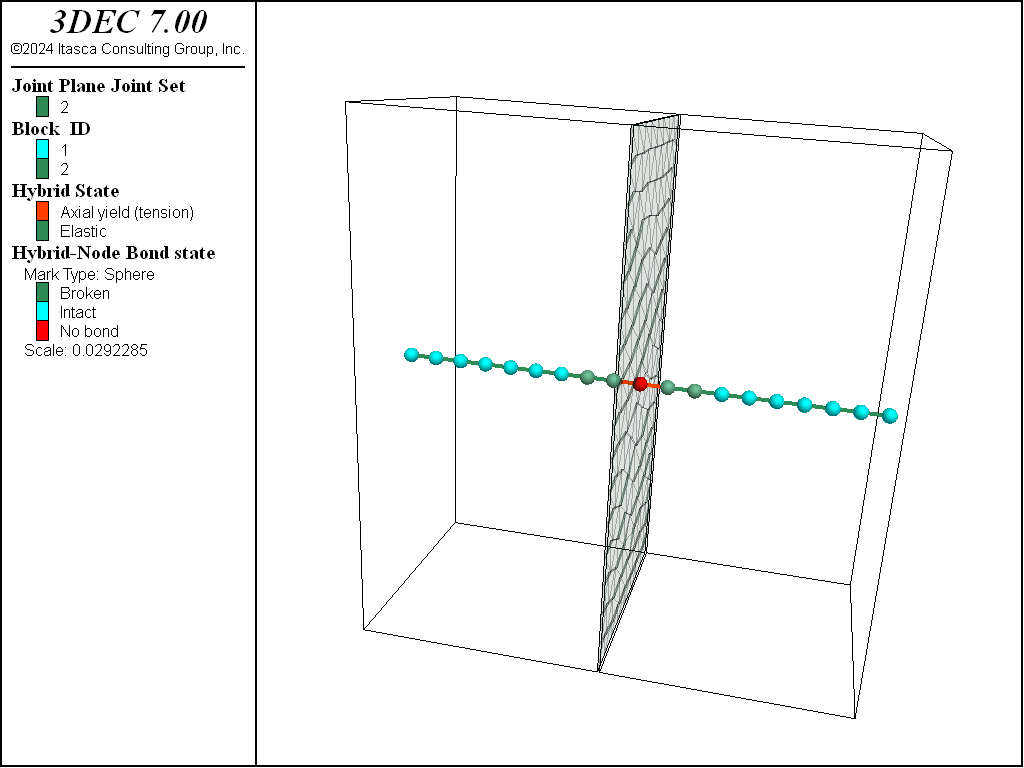
Figure 19: Blocks and bolt configuration in the pullout test. Model is shown after bolt pullout.
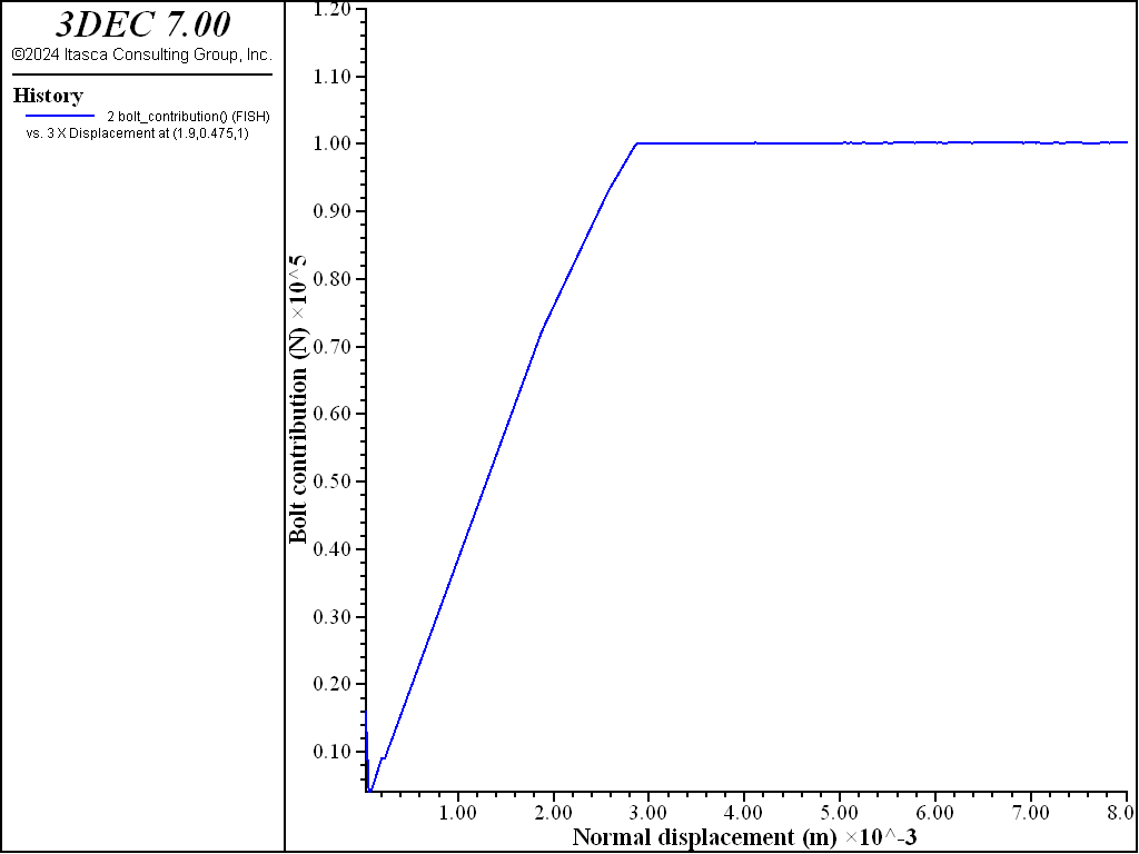
Figure 20: Bolt contribution in the pullout test.
pullout.dat
;;-----------------------------------------------------------------------------
;;		Pull-out test
;;-----------------------------------------------------------------------------
model restore 'blocks'
;
; Define parameters for pullout test
[global xvel_ = 1e-2]
;
block gridpoint apply velocity-x 0 range position-x 0
;
block hide range position-x 0 [block_lenH]
block gridpoint apply velocity-z 0 range position-z 0
block gridpoint group 'right' range pos-x [block_lenH]
block hide off
;
block gridpoint apply velocity-x [xvel_] range group 'right'
;
[global max_force = 0.0]
[global bolt_contribution = 0.0]
;
fish define reaction_force
  local temp_ = 0.0
  loop foreach local gi block.gp.list
    if block.gp.group(gi) = 'right'
        temp_ = temp_ + block.gp.force.reaction.x(gi)
    end_if
  end_loop
  reaction_force = math.abs(temp_)
  bolt_contribution =  math.abs(temp_); - friction_force
end
;
fish history reaction_force
fish history bolt_contribution
block history displacement-x ...
  position [2*block_lenH] [0.5*block_lenH] [0.5*block_lenV]
model history mechanical unbalanced-maximum
history interval 500

;fish function to run the test - stop when rupture
[global gp_monitor = block.gp.near(2*block_lenH,0.5*block_lenH,0.5*block_lenV)]

fish def run_it
  local test_ = true
  loop while test_ = true
    command
model cycle 10000
    end_command
    if math.mag(block.gp.dis(gp_monitor)) > 8e-3
      test_ = false
    endif
  end_loop
end
;
model save 'ini_pull'
;
=================================================================
;
; Test perpendicular bolt 90 degrees
; Change dincl_ to test other bolt angles
;
model restore 'ini_pull'
[global dincl_=90.]

;To create bolt
[global x1 = block_lenH-0.5*bolt_len*math.sin(dincl_*math.degrad)+0.001]
[global y1 = 0.5*block_lenH]
[global z1 = 0.5*block_lenV+0.5*bolt_len*math.cos(dincl_*math.degrad)]
[global x2 = block_lenH+0.5*bolt_len*math.sin(dincl_*math.degrad)-0.001]
[global y2 = y1]
[global z2 = 0.5*block_lenV-0.5*bolt_len*math.cos(dincl_*math.degrad)]
[global bolt_beg=vector(x1,y1,z1)]
[global bolt_end=vector(x2,y2,z2)]

sel hybrid create by-line [bolt_beg] [bolt_end] property 1 ...
  segment-length [segment_length_] dowel-length [dowel_length_]

; cable properties
sel hybrid prop 1  cross-sectional-area [area_] young [e_] ...
  grout-stiffness [grout_stiff_] grout-cohesion [grout_strength_] ...
  yield-tension [cable_yield_] rupture-tension-strain [cable_strain_limit_]

; dowel properties
sel hybrid prop 1 dowel-stiffness [dowel_stiffness_] ...
  dowel-yield [dowel_yield_] dowel-strainlimit [dowel_strain_limit_]

[run_it]

model save 'pull-90'

program return

===============================================================================

;inclined bolt 70 degrees

model restore 'ini_pull'
[global dincl_=70.]

;To create inclined bolt
[global x1 = block_lenH-0.5*bolt_len*math.sin(dincl_*math.degrad)+0.001]
[global y1 = 0.5*block_lenH]
[global z1 = 0.5*block_lenV+0.5*bolt_len*math.cos(dincl_*math.degrad)]
[global x2 = block_lenH+0.5*bolt_len*math.sin(dincl_*math.degrad)-0.001]
[global y2 = y1]
[global z2 = 0.5*block_lenV-0.5*bolt_len*math.cos(dincl_*math.degrad)]
[global bolt_beg=vector(x1,y1,z1)]
[global bolt_end=vector(x2,y2,z2)]

sel hybrid create by-line [bolt_beg] [bolt_end] property 1 ...
  segment-length [segment_length_] dowel-length [dowel_length_]

; cable properties
sel hybrid prop 1  cross-sectional-area [area_] young [e_] ...
  grout-stiffness [grout_stiff_] grout-cohesion [grout_strength_] ...
  yield-tension [cable_yield_] rupture-tension-strain [cable_strain_limit_]

; dowel properties
sel hybrid prop 1 dowel-stiffness [dowel_stiffness_] ...
  dowel-yield [dowel_yield_] dowel-strainlimit [dowel_strain_limit_]

[run_it]

model save 'pull-70'
;------------------------------------------------------------------------------

;end of file
Example Application: Simple Tunnel
A simple circular tunnel with a radius of 1 m is simulated. It is a 2.5D bonded block model (BBM) with a length of 2 m. Quarter symmetry is assumed. This is a bonded block model in which zones are transformed into tetrahedral blocks. A joint set is then imprinted on top of the bonded block assembly.
The tunnel is partially excavated by applying decreasing reaction forces on the tunnel surface, then hybrid bolts are installed before removing the reaction forces. Five hybrid bolts are installed with a length of 4 m. The cable configuration is shown in Figure 21.
The resulting joint shear displacements and shear forces in the dowels are shown in Figure 22.
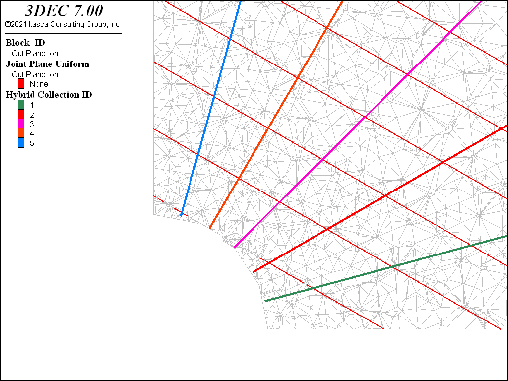
Figure 21: Joints and bolts in a cross-section of the tunnel model.
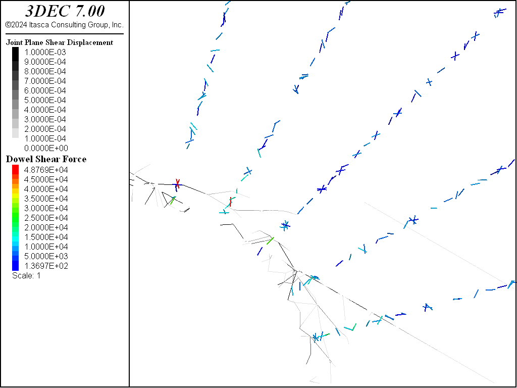
Figure 22: Joint shear displacements and dowel shear forces after solving.
tunnel.dat
; Example simple tunnel supported with hybrid bolts
;
model new
model random 10000
block create tunnel length -1 1 blocks-radial 8 blocks-tangential 2 ...
  boundary 8 radius-ratio 1.1
;
; quarter tunnel
block delete range position-x -100 0
block delete range position-z -100 0
;
block zone generate center 0 0 0 edgelength-center 0.1 distance 9 ...
  edgelength-distance 0.5
;
; dump zones to file as blocks (poly.dat)
block zone list poly

=========================================
model new
model random 10000
model large-strain on
;
block tolerance 0.001
;
program call 'poly'
;
; put in a joint set
block cut joint-set dip 30 dip-direction 90 spacing 0.5 number 20 ...
  jointset-id 999
;
block zone generate center 0 0 0 edgelength-center 0.1 distance 9 ...
  edgelength-distance 0.5
;
block zone cmodel assign elastic
block zone property density 2600 bulk 1e9 shear 3e8

; joints between tets
block contact property stiffness-normal 1e11 stiffness-shear 1e11 ...
  friction 40.0 cohesion 1e3 tension 1e2
;
; faults
block contact property stiffness-normal 1e10 stiffness-shear 1e10 ...
  friction 40.0 range joint-set 999

; new contacts
block contact material-table default property stiffness-normal 1e10 ...
  stiffness-shear 1e10 friction 40.0
;
block gridpoint apply velocity-x 0 range position-x 0
block gridpoint apply velocity-z 0 range position-z 0
block gridpoint apply velocity-x 0 range position-x 9
block gridpoint apply velocity-z 0 range position-z 9
block gridpoint apply velocity-y 0 range position-y -1
block gridpoint apply velocity-y 0 range position-y 1
;
block insitu stress -5e6 -3e6 -3e6 0 0 0
;
model solve
;
model save 'initial'

;model restore 'initial'
;
block group 'rock'
block group 'tunnel' range cylinder end-1 0 -1 0 end-2 0 1 0 radius 1
;
; identify surface of tunnel

; change face group for plotting
block face group 'surface' range group-int 'rock' 'tunnel'

; change gridpoint group for applying reaction forces
block gridpoint group 'surface' range group-int 'rock' 'tunnel'
;
block delete range cylinder end-1 0 -1 0 end-2 0 1 0 radius 1
;
model cycle 1
;
fish define bound_his_ini
  bound_his_start = global.step
end
[bound_his_ini]
;
; function to gradually reduce reaction forces
fish define bound_his
  ; non-linear, approaches 0 in ~ 10000 steps
  bound_his = 0.95^((global.step-bound_his_start)/10.0)
end
;
block gridpoint apply reaction fish bound_his range group 'surface'
fish history bound_his
;
model cycle 1000
;
model save 'pre-bolt'

fish define install_cables
  tol = 0.01
  loop i (1,5)
    angle = math.pi*0.5*i/6.0
    p1x = math.cos(angle)+tol
    p1z = math.sin(angle)+tol
    p2x = 4.0*math.cos(angle)
    p2z = 4.0*math.sin(angle)
    command
      sel hybrid create by-line [p1x],0,[p1z]  [p2x],0,[p2z] ...
                        prop 1 seg 20 dowel-len 0.025
    end_command

  end_loop
end
[install_cables]
;
; cable properties
sel hybrid property 1 cross-sectional-area 181e-6 young 98.6e11 ...
   yield-tension 5e6 grout-stiffness 1.12e9 grout-cohesion 1.75e9

; dowel properties
sel hybrid property 1 dowel-stiffness 2e10 dowel-yield 5e5 ...
  dowel-strainlimit 0.015
;
model solve ratio 1e-5 or cycles 5000
model save 'hybrid'
;
Modeling Considerations
Material Properties
Property numbers are assigned to reinforcement or hybrid bolt elements with the property keyword when they are created (sel reinforcement create, sel hybrid create). It should be noted that all quantities must be given in an equivalent set of units (see Table 6). Note that for reinforcement or hybrid bolt elements, stiffness has units of [force/displacement] and strength has units of [force].
| Property | Unit | SI | Imperial | ||||
|---|---|---|---|---|---|---|---|
| Area | length2 | m2 | m2 | m2 | cm2 | ft2 | in2 |
| Bond Stiffness | force/length/disp | N/m/m | kN/m/m | MN/m/m | Mdynes/cm/cm | lbf/ft/ft | lbf/in/in |
| Bond Strength | force/length | N/m | kN/m | MN/m | Mdynes/cm | lbf/ft | lbf/in |
| Density | mass/volume | kg/m3 | 103 kg/m3 | 106 kg/m3 | 106 g/m3 | lbf/ft2 | psi |
| Elastic Modulus | stress | Pa | kPa | MPa | bar | lbf/ft2 | psi |
| Stiffness | force/disp | N/m | kN/m | MN/m | Mdynes/cm | lbf/ft | lbf/in |
| Yield Strength | force | N | kN | MN | Mdynes | lbf | lbf |
Symmetry Conditions
Structural elements that lie on a plane of symmetry should be assigned full properties for modulus and stiffness. Property values for cross-sectional area and yield strength should be reduced by 50% compared to the same property values for elements not on the symmetry plane. Loads applied to structural elements on symmetry planes should also be reduced by 50% compared to the same loads applied away from the symmetry plane.
Equilibrium Conditions
The user must decide when the model has reached an equilibrium state. Equilibrium for problems involving structural elements can be determined by all the usual criteria (e.g., histories, velocity fields).
Sign Convention
Axial forces in all structural elements are positive in compression. Shear forces follow the opposite sign convention as that given for zone shear stresses. Axial displacements for hybrid bolt elements are positive for loading in compression. Axial displacements for local reinforcement elements are positive for loading in tension.
References
Bjurstrom, S. “Shear Strength on Hard Rock Joints Reinforced by Grouted Untensioned Bolts,” in Proceedings of the 3rd International Congress on Rock Mechanics, Vol. II, Part B, pp. 1194-1199. Washington, D.C.: National Academy of Sciences (1974).
Dight, P. M. “Improvements to the Stability of Rock Walls in Open Pit Mines.” Ph.D. Thesis, Monash University (1982).
Fuller, P. G., and R. H. T. Cox. “Rock Reinforcement Design Based on Control of Joint Displacement — A New Concept,” in Proceedings of the 3rd Australian Tunnelling Conference (Sydney, Australia, 1978), pp. 28-35. Sydney: Inst. of Engrs., Australia (1978).
Gerdeen, J. C., et al. “Design Criteria for Roof Bolting Plans Using Fully Resin-Grouted Nontensioned Bolts to Reinforce Bedded Mine Roof,” U.S. Bureau of Mines, OFR 46(4)-80 (1977).
Haas, C. J. “Shear Resistance of Rock Bolts,” Trans. Soc. Min. Eng. AIME, 260(1), 32-41 (1976).
Hyett, A. J., W. F. Bawden and R. D. Reichert. “The Effect of Rock Mass Confinement on the Bond Strength of Fully Grouted Cable Bolts,” Int. J. Rock Mech. Min. Sci. & Geomech. Abstr., 29(5), 503-524 (1992).
Itasca Consulting Group Inc. UDEC (Universal Distinct Element Code), Version 5.0. Minneapolis: ICG (2011).
Littlejohn, G. S., and D. A. Bruce. “Rock Anchors – State of the Art. Part I: Design,” Ground Engineering, 8(3), 25-32 (1975).
Lorig, L. J. “A Simple Numerical Representation of Fully Bonded Passive Rock Reinforcement for Hard Rocks,” Computers and Geotechnics, 1, 79-97 (1985).
Par Un Groupe Francais (Azuar, Debreuille, Habib, Londe, Panet and Salembier). “Le Renforcement des Massifs Rocheux par Armatures Passives (Rock Mass Reinforcement by Passive Rebars),” in Proceedings of the 4th ISRM Congress (Montreux, Switzerland, September 1979), Vol. 1, pp. 23-30. Rotterdam: A. A. Balkema and The Swiss Society for Soil and Rock Mechanics (1979).
Pells, P. J. N. “The Behaviour of Fully Bonded Rock Bolts,” in Proceedings of the 3rd International Congress on Rock Mechanics, Vol. 2, pp. 1212-1217 (1974).
St. John, C. M., and D. E. Van Dillen. “Rockbolts: A New Numerical Representation and Its Application in Tunnel Design,” Rock Mechanics – Theory - Experiment - Practice (Proceedings of the 24th U.S. Symposium on Rock Mechanics, Texas A&M University, June, 1983), pp. 13-26. New York: Association of Engineering Geologists (1983).
| Was this helpful? ... | 3DEC © 2019, Itasca | Updated: Feb 25, 2024 |