Calculation Modes for Fluid-Mechanical Interaction
The calculation mode and commands required for a pore-pressure analysis
depend on whether the grid has been configured for fluid flow
(i.e., whether the model configure fluid command has been specified).
The flow calculation can be performed independent of, or coupled to,
the mechanical deformation calculation when model configure fluid is specified.
It is also possible to conduct simplified, uncoupled, fluid-mechanical calculations with FLAC3D such as slope stability analyses, without configuring the grid for fluid flow. This option, when applicable, provides faster solution than the fluid flow configuration.
Grid Not Configured for Fluid Flow and Grid Configured for Fluid Flow reflect the two possibilities. For convenience, all commands described below are summarized in Input Instructions for Fluid-Flow Analysis, at the end of this section.
Grid Not Configured for Fluid Flow
If the command model configure fluid has not been given,
then a fluid-flow analysis cannot be performed,
but it is still possible to assign pore pressure at gridpoints.
In this calculation mode, pore pressures do not change, but failure,
which is controlled by the effective-stress state,
may be induced when plastic constitutive models are used.
A pore-pressure distribution can be specified at gridpoints,
with the zone gridpoint initialize pore-pressure command with a gradient,
or with the zone water plane (or zone water set) command.
If the zone water plane command is used,
a hydrostatic pore-pressure distribution is calculated automatically by the code,
below the given water table level.
In this case, the fluid density
(zone water density) and gravity (model gravity) must also be specified.
The fluid density value and water table location can be printed with the zone list fluid-density command,
and the water table can be plotted,
if the water table is defined by zone water set or zone water plane command.
In both cases, zone pore pressures are calculated by averaging from the gridpoint values,
and used to derive effective stresses for use in the constitutive models.
In this calculation mode, the fluid presence is not automatically accounted for in the calculation of body forces:
wet and dry medium densities must be assigned by the user, below and above the water level, accordingly.
The commands zone gridpoint list pore-pressure and zone list pore-pressure print gridpoint and zone pore pressures, respectively.
plot add zone contour pore-pressure plots contours of gridpoint pore pressures.
A simple example application of this calculation mode is given in the topic The Effect of Water in the Problem Solving section.
Grid Configured for Fluid Flow
If the command model configure fluid is given, a transient fluid-flow analysis can be performed,
and change in pore pressures,
as well as change in the phreatic surface, can occur.
Pore pressures are calculated at gridpoints, and zone values are derived using averaging.
Both effective-stress (static pore-pressure distribution)
and undrained calculations can be carried out in model configure fluid mode.
In addition, a fully coupled analysis can be performed,
in which changes in pore pressure generate deformation,
and volumetric strain causes the pore pressure to evolve.
If the grid is configured for fluid flow, dry densities must be assigned by the user (both below and above the water level), because FLAC3D takes the fluid influence into account in the calculation of body forces.
A fluid-flow model must be assigned to zones when running in model configure fluid mode.
Isotropic flow is prescribed with the zone fluid cmodel assign isotropic command;
anisotropic flow with the command zone fluid cmodel assign anisotropic.
An impermeable material is assigned to zones with the zone fluid cmodel assign null command.
Note that zones that are made null mechanically are not automatically made null for fluid flow.
Fluid properties are assigned to either zones or gridpoints.
Zone fluid properties include isotropic permeability, porosity, Biot coefficient, undrained thermal coefficient and fluid density.
Zone fluid properties are assigned with the zone fluid property command, with the exception of fluid density,
which is assigned with the zone initialize fluid-density command.
(Note that fluid density can also be specified globally with the zone water density command.)
For isotropic flow, permeability is specified using the permeability property keyword. For anisotropic flow, the three principal values of permeability are specified using the property keywords permeability-1, permeability-2 and permeability-3, and the orientation is defined using the keywords dip, dip-direction, and rotation. The principal directions of permeability correspond to \(k_1\), \(k_2\), \(k_3\), and form a right-handed system. The properties dip and dip-direction are the dip angle and dip direction angle of the plane in which \(k_1\) and \(k_2\) are defined. The dip angle is measured from the global \(xy\)-plane, positive down (in negative \(z\)-direction). The dip direction angle is the angle between the positive \(y\)-axis and the projection of the dip-direction vector on the \(xy\)-plane (positive clockwise from \(y\)-axis). The property rotation is the rotation angle between the \(k_1\)-axis and the dip vector in the \(k_1\)-\(k_2\)-plane (positive clockwise from dip-direction vector). See Figure 1.
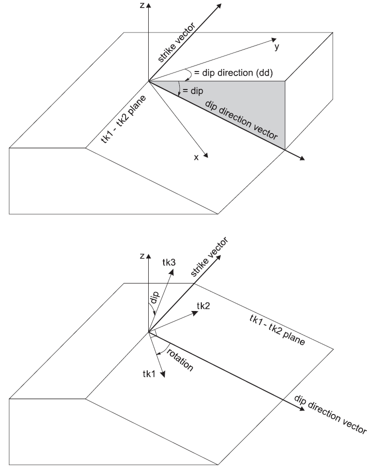
Figure 1: Definitions for principal directions of permeability tensor.
Biot coefficient is assigned using the biot keyword; porosity is assigned using the porosity keyword. If not specified, Biot coefficient = 1 and porosity = 0.5, by default.
Gridpoint fluid properties are assigned with the zone gridpoint initialize command.
These properties include fluid bulk modulus, Biot modulus, fluid tension limit and saturation.
Each of the gridpoint properties can also be given a spatial variation.
Table 1 summarizes the ways the various properties can be specified. The fluid properties are described further in Properties and Units for Fluid-Flow Analysis.
| property | keyword | specific | command |
|---|---|---|---|
| Permeability (isotropic) | permeability | in zones | zone fluid property permeability |
| Perm. princ. val. (aniso) | permeability-1 | in zones | zone fluid property permeability-1 |
| Perm. princ. val. (aniso) | permeability-2 | in zones | zone fluid property permeability-2 |
| Perm. princ. val. (aniso) | permeability-3 | in zones | zone fluid property permeability-3 |
| Perm. princ. val. (aniso) | permeability-xx | in zones | zone fluid property permeability-xx |
| Perm. princ. val. (aniso) | permeability-xy | in zones | zone fluid property permeability-xy |
| Perm. princ. val. (aniso) | permeability-xz | in zones | zone fluid property permeability-xz |
| Perm. princ. val. (aniso) | permeability-yy | in zones | zone fluid property permeability-yy |
| Perm. princ. val. (aniso) | permeability-yz | in zones | zone fluid property permeability-yz |
| Perm. princ. val. (aniso) | permeability-zz | in zones | zone fluid property permeability-zz |
| Perm. princ. dir. (aniso) | dip | in zones | zone fluid property dip |
| Perm. princ. dir. (aniso) | did-direction | in zones | zone fluid property dip-direction |
| Perm. princ. dir. (aniso) | rotation | in zones | zone fluid property rotation |
| Porosity | porosity | in zones | zone fluid property porosity |
| Biot coefficient | biot | in zones | zone fluid property biot |
| Undrained thermal coeff. | undrained-thermal-coefficient | in zones | zone fluid property undrained-thermal-coefficient |
| Fluid modulus | fluid-modulus | at gridpoints | zone gridpoint initialize fluid-modulus |
| Biot modulus | biot-modulus | at gridpoints | zone gridpoint initialize biot-modulus |
| Saturation | saturation | at gridpoints | zone gridpoint initialize saturation |
| Fluid tension limit | fluid-tension | at gridpoints | zone gridpoint initialize fluid-tension |
| Fluid density | fluid-density | at zones | zone initialize fluid-density |
| density | globally | zone water density |
Note that fluid compressibility is defined in one of two ways in the model configure fluid mode:
1) Biot coefficient and Biot modulus are specified; or
2) fluid bulk modulus and porosity are specified.
The first case accounts for the compressibility of the solid grains
(Biot coefficient is set to 1 for incompressible grains).
In the second case, solid grains are assumed to be incompressible
(see Biot Coefficient and Biot Modulus).
The zone properties can be printed with the zone fluid list property command,
and the gridpoint properties can be printed with the zone gridpoint list command.
Fluid density, along with the location of the water table (if specified) can be printed with the zone water list command.
The fluid-flow properties can be plotted as a contour plot.
For anisotropic flow, the global components of the permeability tensor are available for plotting and printing,
using the zone property keywords
permeability-xx,
permeability-yy,
permeability-zz,
permeability-xy,
permeability-xz and
permeability-zz
(please note that these global components cannot be initialized directly).
An initial gridpoint pore-pressure distribution is assigned the same way
for the model configure fluid mode as for the non-model configure fluid mode
(i.e., either with the zone gridpoint initialize pore-pressure command
or the zone water set or zone water plane command).
Pore pressures can be fixed (and freed) at selected gridpoints with the zone gridpoint fix pore-pressure
(or zone gridpoint free pore-pressure) command.
Fluid sources and sinks can be applied with the zone apply well command.
See describes the various Fluid-Flow Boundary and Initial Conditions.
The fluid-flow solution is controlled by the zone fluid active on and model solve commands.
Several keywords are available to help the solution process.
For example, zone fluid active on or off turns on or off the fluid flow calculation mode.
The application of these commands and keywords depends on the level of coupling required in the fluid flow analysis.
The section in Solving Flow-Only and Coupled-Flow Problems
describes the various coupling levels and the recommended solution procedure.
Example applications, ranging from flow-only to coupled mechanical-flow calculations, are also described in this section.
Results from a fluid-flow analysis are provided in several forms.
The commands zone gridpoint list pore-pressure and zone list pore-pressure print gridpoint and zone pore pressures, respectively.
Histories of gridpoint and zone pore pressures can be monitored
with the command zone history pore-pressure and specify source.gridpoint and source.zone, respectively.
And for a transient calculation, the pore pressure can be plotted versus real time
by monitoring the flow time with the model history fluid time-total command.
plot add zone contour pore-pressure plots contours of gridpoint pore pressures.
plot add zone contour saturation plots contours of saturation.
The plot add flow command plots specific discharge vectors.
General information on the model configure fluid calculation mode is printed with the model fluid list command.
Several fluid-flow variables can be accessed through FISH.
These are listed in Input Instructions for Fluid-Flow Analysis.
There is one grid-related variable, gp.flow, that can only be accessed through a FISH function;
this corresponds to the net inflow or outflow at a gridpoint.
The summation of such flows along a boundary where the pore pressure is fixed is useful
because it can provide a value for the total outflow or inflow for a system.
| Was this helpful? ... | 3DEC © 2019, Itasca | Updated: Feb 25, 2024 |