FLAC3D Theory and Background • Fluid-Mechanical Interaction

Pressuremeter Test

Note

The project file for this example is available to be viewed/run in FLAC3D.[1] The project’s main data files are shown at the end of this example.

The pressuremeter test is used to determine in-situ mechanical properties of soils (Wood 1990). A long, rubber membrane is expanded against the walls of a vertical borehole (Figure 1). The pressure inside the membrane is constant. Radial displacements of the borehole wall are measured as a function of the pressure. The soil deforms in plane strain in the plane normal to the borehole and sufficiently distant from the ends of the membrane.

The borehole (radius \(a\) = 0.03 m) is drilled in homogeneous, isotropic soil. The soil is assumed to behave as a linearly elastic material saturated with groundwater. Several mechanical properties of the soil and groundwater are assumed in this problem:

shear modulus (\(G\))	11.1 MPa
bulk modulus (\(K\))	33.3 MPa
porosity (\(n\))	0.48
soil permeability (\(k\))	1.02 × 10-14 \({m^2}\over{Pa-sec}\)
bulk modulus of water (\(K_f\))	500 MPa

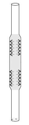
Figure 1: Cylindrical cavity expansion in pressuremeter test.

The initial state of (total) stress in the soil is isotropic: \(\sigma_1=\sigma_2=\sigma_3\) = -327.87 kPa, while the initial pore pressure is \(p=p_i\) = 147.0 kPa.

The soil is allowed to consolidate for 300 seconds after the drilling of the borehole. After the consolidation, the pressure inside the rubber membrane is increased from zero to 1 MPa during 600 seconds. (The rubber membrane prevents further drainage of the groundwater into the borehole.)

The analytical solution for two-dimensional consolidation of a borehole in an elastic medium was obtained by Detournay and Cheng (1988). The drilling of the borehole is simulated by removing the stress acting on the inner boundary of the borehole and setting the pore pressure to zero at time \(t\) = 0. Since the initial stress is isotropic, the loading conditions can be decomposed into two modes: (1) mode 1, an isotropic stress; and (2) mode 2, an initial pore-pressure distribution. The boundary conditions at the wall of the borehole for each loading mode can be expressed:

1. mode 1

\[\begin{split}\begin{split} \sigma_{rr} &= -\sigma_i \\ \sigma_{r\theta} &= 0 \\ p &= 0 \end{split}\end{split}\]

2. mode 2

\[\begin{split}\begin{split} \sigma_{rr} &= 0 \\ \sigma_{r\theta} &= 0 \\ p &= -p_i \end{split}\end{split}\]

The stresses and displacements due to mode 1 loading are described by the classical Lamé solution. Because the volumetric strain computed from the Lamé solution is zero throughout the domain, the mode 1 loading does not generate pore pressure, and deformation takes place instantaneously. The evolution of the pore-pressure field due to mode 2 loading is governed by a homogeneous diffusion equation. The deformation and stress fields can be calculated from the pore-pressure field. The problem is solved in the Laplace transform domain, and the solutions are transformed back to the time domain using the numerical inversion method developed by Stehfest (1970). The complete solution is described by Detournay and Cheng (1988). The analytical solutions are calculated and imported into FLAC3D tables for comparison to the numerical results.

Because the problem is axisymmetric, it is simulated using a row of 61 zones forming a truncated wedge of 9° angle. The geometry of the model and boundary conditions are illustrated in Figure 2. The FLAC3D grid is shown in Figure 3. The far-field boundary is at radius \(b\) = 1.50 m and can be considered at infinity if radius \(b\) is scaled to the radius of the borehole (\(a\) = 0.03 m). (The length resulting from the diffusivity of the model and time of the simulation are also much smaller than \(b\).)

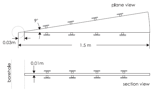
Figure 2: Domain of FLAC3D simulation.

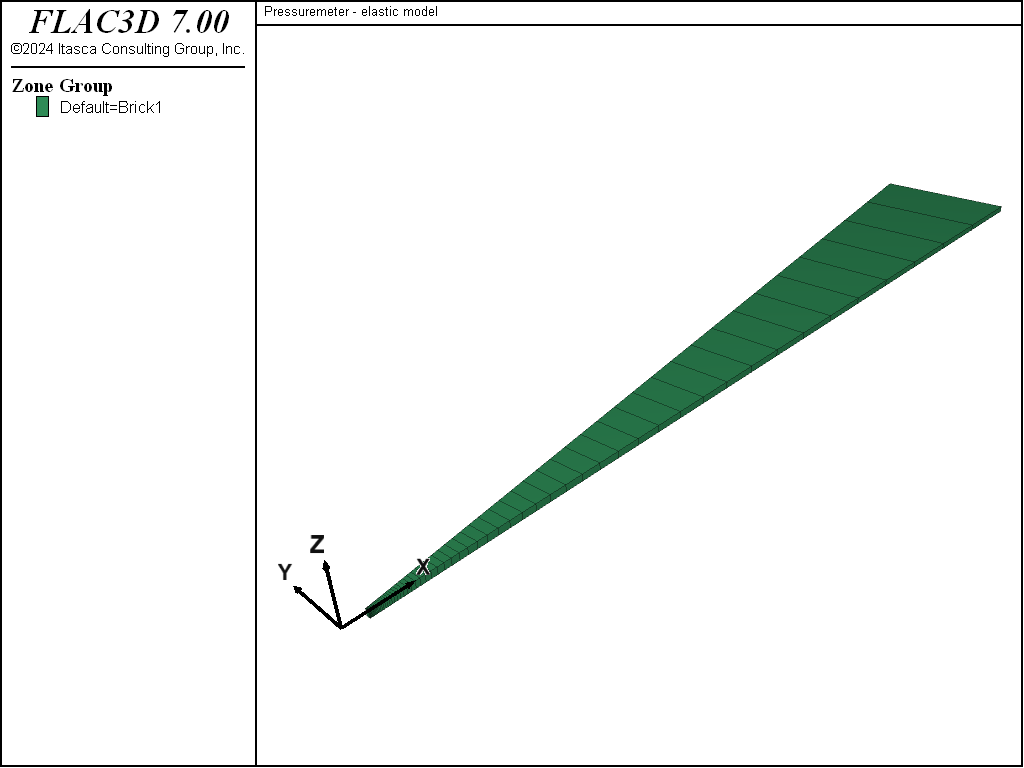
Figure 3: FLAC3D grid.

break

The simulation is conducted in the steps corresponding to the actual operations in the field test:

(1) The total stress on the contour of the borehole is reduced to zero, simulating drilling of the borehole. Although the total stress (in the FLAC3D model) is reduced to zero in steps, the change in real flow time is instantaneous (i.e., the model undergoes undrained deformation). (The fluid flow calculation is turned off: model fluid active off.) The model is iterated to reach mechanical equilibrium.

(2) The pressure boundary condition at the contour of the borehole is set to zero. The model consolidates for 300 seconds (model fluid active on), resulting in the drainage of the groundwater into the borehole.

(3) The contour of the borehole is defined as impervious (due to installation of the rubber membrane), and the pressure boundary condition is applied on the contour of the borehole: 1.0 MPa in 100 increments at each 6 seconds. That is, the soil consolidates under the applied load for 6 seconds before the next load increment (0.01 MPa) is applied.

The profiles of the normalized pore pressure, \(p/p_i\), normalized radial stress, \(\sigma_{rr}/\sigma_i\), and tangential stress, \(\sigma_{\theta\theta}/\sigma_i\) (as a function of the normalized radius \(r/a\)), after 300 seconds of consolidation, calculated from FLAC3D and using the closed-form solution from Detournay and Cheng (1988), are shown in Figure 4 and Figure 5. Agreement between the curves is very good.

The profiles of the normalized pore pressures, and the radial and tangential stresses after 600 seconds of pressurization of the borehole are shown in Figure 6 and Figure 7.

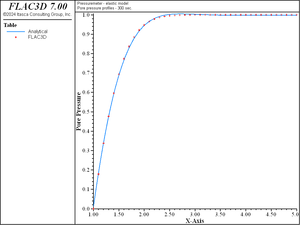
Figure 4: Pore-pressure profiles—300 seconds consolidation.

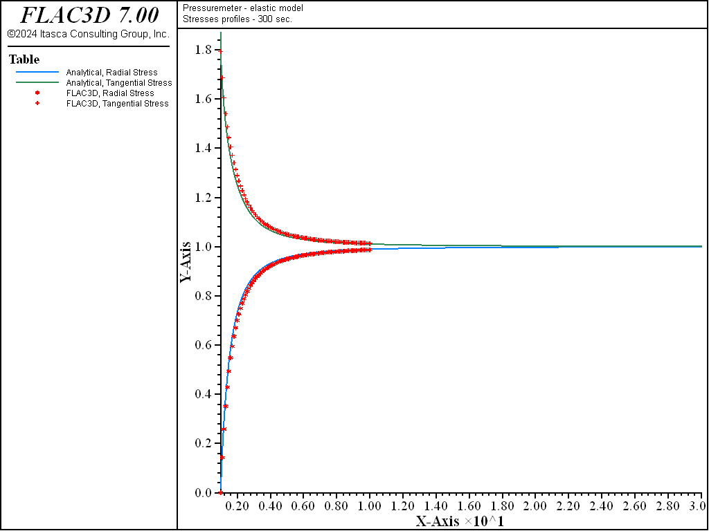
Figure 5: Profiles of radial and tangential normal stresses—300 seconds consolidation.

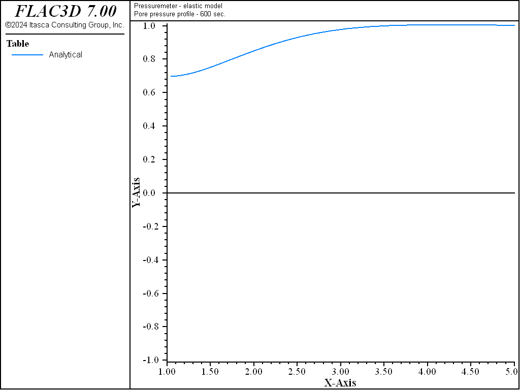
Figure 6: Pore-pressure profiles—600 seconds consolidation.

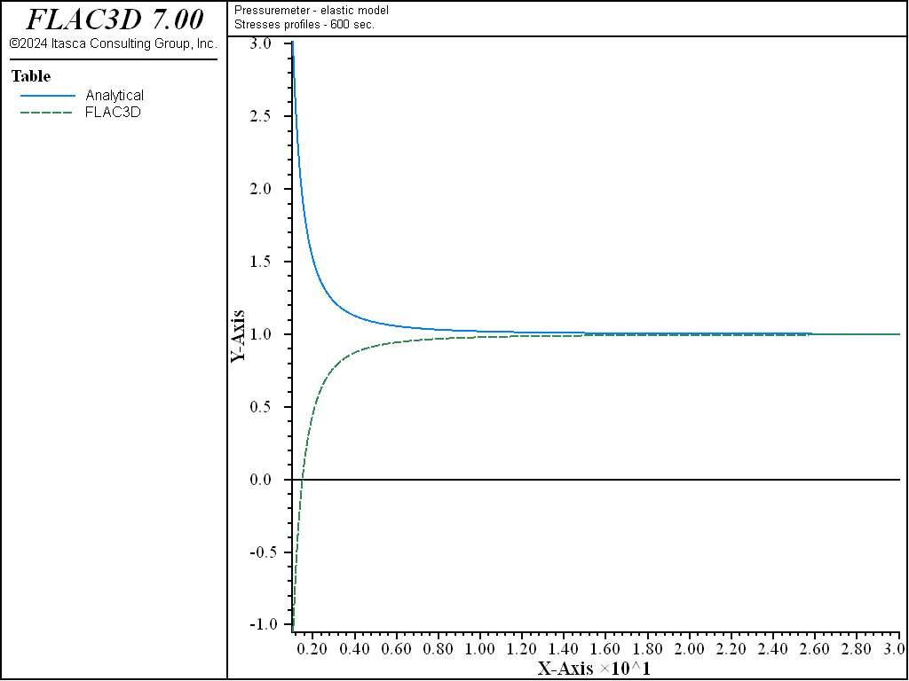
Figure 7: Profiles of radial and tangential normal stresses—600 seconds consolidation.

The pressure variations in the pressuremeter test are often such that nonlinear, plastic deformations are induced in a soil. Therefore, the same problem is simulated using a Mohr-Coulomb model for plastic deformation of the soil. Three parameters are assumed in the simulation:

friction angle (\(\phi\))	22°
dilation angle (\(\psi\))	10°
cohesion (\(c\))	26 kN/m2

The profiles of the normalized pore pressures, and the normalized radial and tangential stresses after 600 seconds of pressurization of the borehole in a Mohr-Coulomb material, are shown in Figure 8 and Figure 9.

The numerical solution for a linearly elastic material is generated using the data file listed in “Pressuremeter-Elastic.dat”. The input data file for a Mohr-Coulomb material is the same, except that (1) the material model is declared a Mohr-Coulomb material (zone cmodel assign mohr-coulomb), and (2) the corresponding material properties are added (zone property bulk 3.33e7 shear 1.11e7 friction 30 dilation 10 cohesion 26000). The data file “fishFunctions” generates the tables with the profiles of the normalized pore pressure and the normalized stresses (see “Pressuremeter-MC.dat”). The data file “preana” contains tables in which the analytical elastic solutions for pore pressure, radial and tangential stress profiles after 300 seconds of pressurization are stored.

break

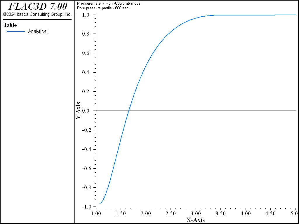
Figure 8: Pore-pressure profile—600 seconds consolidation (Mohr-Coulomb material).

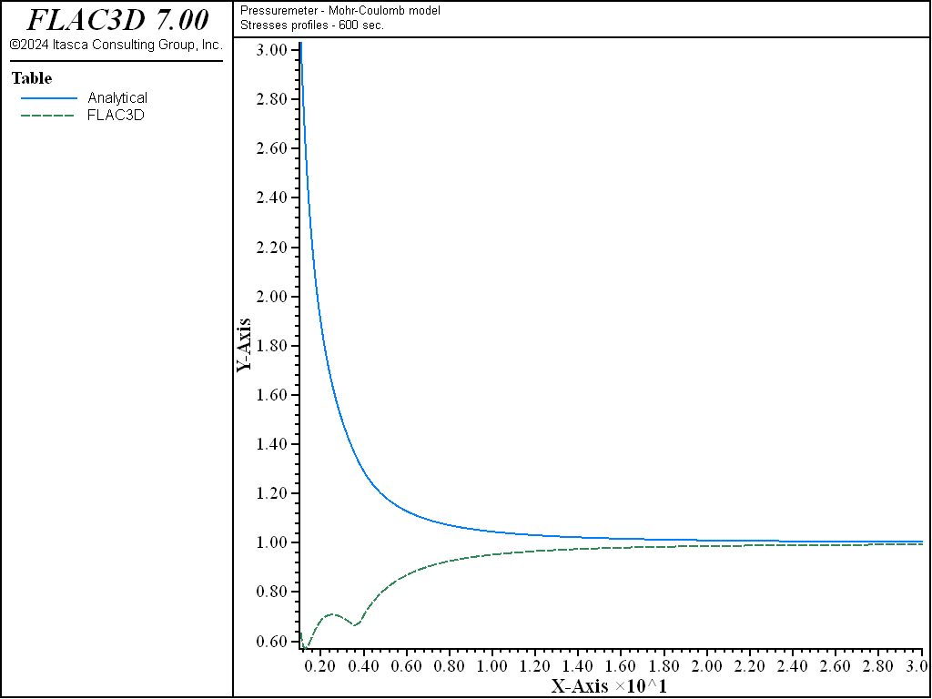
Figure 9: Profiles of radial and tangential normal stresses—600 seconds consolidation (Mohr-Coulomb material).

References

Detournay, E., and A. H. D. Cheng. “Poroelastic Response of a Borehole in a Non-Hydrostatic Stress Field,” Int. J. Rock Mech. Sci. & Geomech. Abstr., 25(3), 171-182 (1988).

Stehfest, H. “Numerical Inversion of Laplace Transforms,” Communic. Ass. Comput. Mach., 13, 47-49 (1970).

Wood, D. M. Soil Behaviour and Critical State Soil Mechanics. Cambridge: Cambridge University Press (1990).

Data Files

Pressuremeter-Elastic.dat

;   pressuremeter test in poro-elastic material, (a) Elastic model
model new
model title 'Pressuremeter - elastic model'
fish automatic-create off
program call 'fishFunctions' suppress
[global time0 = time.clock]
model configure fluid
zone create brick point 0 (0.03,0,0)       point 1 (1.5,0,0) ...
                  point 2 (0.03,0,-0.01)   point 4 (1.5,0,-0.01) ...
                  point 3 (2.96307e-2,0.46930e-2,0) ...
                  point 6 (1.48153,0.23465,0) ...
                  point 5 (2.96307e-2,0.46930e-2,-0.01) ...
                  point 7 (1.48153,0.23465,-0.01) ...
                  size 61 1 1 ratio 1.1 1 1
zone face skin
; --- mechanical model, elastic ---
zone cmodel assign elastic
zone property bulk 3.33e7 shear 1.11e7
zone initialize stress xx -327870 yy -327870 zz -327870
; --- gw model ---
zone fluid cmodel assign isotropic
zone fluid biot on
zone fluid property permeability 1.02e-14
zone gridpoint initialize biot [5.0e8/0.48]
zone gridpoint initialize pore-pressure 147000
; -- boundary conditions for all but 'West' stress
zone face apply stress-normal -327870 range group 'East'
zone gridpoint fix pore-pressure  range group 'West'
zone face apply velocity-normal 0 range group 'North'
zone face apply velocity-normal 0 range group 'South'
zone face apply velocity-normal 0 range group 'Top'
zone face apply velocity-normal 0 range group 'Bottom'
; --- excavate: reduction of total pressure to zero in steps ---
[global factor = 0.99]
fish define slow_excav
    if zone.mech.ratio < 1e-5 then
        factor = math.max(0, factor - 0.0001)
    endif
    slow_excav = factor
end
zone face apply stress-normal -327870 fish slow_excav range group 'West'
model fluid active off
model large-strain on
model solve ratio 3e-6
model save 'pre1'
; --- let water flow out for 300 s ---
model fluid active on
zone gridpoint initialize pore-pressure 0 range group 'West'
model fluid substep 10
model mechanical substep 40000
model mechanical slave on
model solve fluid time-total 300 or mechanical ratio 3e-6
model save 'pre2'
; --- apply pressure inside the borehole ---
zone gridpoint free pore-pressure range group 'West'
fish define charge
    charge = math.max(0.0,fluid.time.total-300.0) / 600.0
end
zone face apply stress-normal -1e6 fish charge range group 'West'
model mechanical substep 40000
model mechanical slave on
model fluid active on
model solve fluid time-total 900 or mechanical ratio 3e-6
[global time = (time.clock-time0)/100.0]
fish list [time]
model save 'pre3'

break

Pressuremeter-MC.dat

;   pressuremeter test in poro-elastic material, (b) Mohr-Coulomb model
model new
model title 'Pressuremeter - Mohr-Coulomb model'
fish automatic-create off
program call 'fishFunctions' suppress
[global time0=time.clock]
model configure fluid
zone create brick point 0 (0.03,0,0)     point 1 (1.5,0,0) ...
                  point 2 (0.03,0,-0.01) point 4 (1.5,0,-0.01) ...
                  point 3 (2.96307e-2,0.46930e-2,0) ...
                  point 6 (1.48153,0.23465,0) ...
                  point 5 (2.96307e-2,0.46930e-2,-0.01) ...
                  point 7 (1.48153,0.23465,-0.01) ...
                  size 61 1 1 ratio 1.1 1 1
zone face skin
; --- mechanical model, Mohr-Coulomb ---
zone cmodel assign mohr-coulomb
zone property bulk 3.33e7 shear 1.11e7 friction 30 dilation 10 cohesion 26000
zone initialize stress xx -327870 yy -327870 zz -327870
; --- gw model ---
zone fluid cmodel assign isotropic
zone fluid biot on
zone fluid property permeability 1.02e-14
zone gridpoint initialize biot [5.0e8/4.8]
zone gridpoint initialize pore-pressure 147000
; -- boundary conditions for all but 'West' stress
zone face apply stress-normal -327870 range group 'East'
zone gridpoint fix pore-pressure range group 'West'
zone face apply velocity-normal 0 range group 'North'
zone face apply velocity-normal 0 range group 'South'
zone face apply velocity-normal 0 range group 'Top'
zone face apply velocity-normal 0 range group 'Bottom'
; --- excavate: reduction of total pressure to zero in steps ---
[global factor=0.99]
fish define slow_excav
    if zone.mech.ratio<1e-5 then
        factor = math.max(0,factor - 0.0001)
    endif
    slow_excav = factor
end
zone face apply stress-normal -327870 fish slow_excav range group 'West'
model fluid active off
model large-strain on
model solve ratio 3e-6
model save 'prm1'
; --- let water flow out for 300 s ---
model fluid active on
zone gridpoint initialize pore-pressure 0 range group 'West'
model mechanical substep 40000
model mechanical slave
model solve fluid time-total 300 or mechanical ratio 3e-6
model save 'prm2'
; --- apply pressure inside the borehole ---
zone gridpoint free pore-pressure range group 'West'
fish define charge
    charge = math.max(0.0,fluid.time.total-300.0) / 600.0
end
zone face apply stress-normal -1e6 fish charge range group 'West'
model mechanical substep 40000
model mechanical slave on
model fluid active on
model solve fluid time-total 900 or mechanical ratio 3e-6
[global time = (time.clock-time0)/100.0]
fish list [time]
[maket]
table '1' label 'num. pp   t=600s'
table '2' label 'num. sigr t=600s'
table '3' label 'num. sigt t=600s'
table '4' label 'num. sigz t=600s'
model save 'prm3'

Endnotes

[1]	To view this project in FLAC3D, use the program menu. Help ▼ Examples…   ⮡   FLAC     ⮡   Fluid       ⮡   Pressuremeter         ⮡   Pressuremeter.prj