Hydraulic Fracture with DFN
Note
The project file for this example may be viewed/run in 3DEC.[1] The main data files used are shown at the end of this example.
Introduction
This tutorial will introduce the user to the necessary order of commands for creating a basic hydraulic fracturing model. A discrete fracture network (DFN) is required for this model and is supplied as a supplementary file “dfn.dat”. An additional file (“hf.fis”), including several functions supporting the hydraulic fracture simulation, is also supplied. It appears at the end of this tutorial.
Warning
This problem takes a long time to run. When running this verification problem, allow 12-24 hours (depending on computer speed) for the calculation to complete.
Model Creation
Geometry
First, the model information is cleared and a fluid flow calculation mode is activated with model configure fluid. This command must be applied prior to creating any blocks, to enable memory allocation for calculations of fracture fluid flow. Note also that joint fluid flow in 3DEC requires small strain analysis, so the command model large-strain off is also required.
Next, a FISH function is defined and called to set up parameters that define the model geometry. A centroid of the entire model, located at (0, 0, 0), is specified (xmiddle, ymiddle, zmiddle) and is used for creating a reference point for the boundary points forming the rock body. The extents of the model are also specified (_modelSize_x = 800, _modelSize_y = 800, _modelSize_z = 200). A joint ID for the hydraulic fracture is specified (hf_id=10000). A smaller inner box required for the DFN region is specified by six points (x1, x2, x3, y1, y2, y3, z1, z2, z3) while the extended model is specified by similar variables with a “_ext” suffix. This is done so that the model boundaries are far from the area of interest. Calculations are included in the function to define the area of interest and the limits of the extended model. Additional \(z\)-coordinates are specified (z_sub1, z_sub2) for locations of extra planes of interest. Finally, a zone size is defined (edge_size) for discretization of the inner and outer regions (inner = 10, outer = 3 × inner).
fish define set_geometry

  ; INPUTS

  ; middle of model
  global xmiddle = 0.0
  global ymiddle = 0.0
  global zmiddle = 0.0

  ; size of area of interest (dfn region)
  local _modelSize_x =800
  local _modelSize_y =800
  local _modelSize_z =200

  ; hydraulic fracture joint id
  global hf_id=10000

  ; zone size in area of interest
  global edge_size=10

  ; GEOMETRY CALCULATIONS.  DO NOT CHANGE
  ; limits of area of interest (dfn region)
  global x1 = xmiddle - 0.5*_modelSize_x
  global x2 = xmiddle + 0.5*_modelSize_x
  global y1 = ymiddle - 0.5*_modelSize_y
  global y2 = ymiddle + 0.5*_modelSize_y
  global z1 = zmiddle - 0.5*_modelSize_z
  global z2 = zmiddle + 0.5*_modelSize_z

  ; limits of extended model
  global x1_ext = xmiddle - _modelSize_x
  global x2_ext = xmiddle + _modelSize_x
  global y1_ext = ymiddle - _modelSize_y
  global y2_ext = ymiddle + _modelSize_y
  global z1_ext = zmiddle - _modelSize_z
  global z2_ext = zmiddle + _modelSize_z

  ; z coordinates for extra planes
  global z_sub1 = zmiddle - 0.25*_modelSize_z
  global z_sub2 = zmiddle + 0.25*_modelSize_z

  global edge_size_outer = 3*edge_size ; outer domain discretization
end
Block Model
We initialize a general tolerance for the model (02) that sets minimum distances between grid points and areas of subcontacts, among other settings.
A block model is then created using the following command. The command uses points defined in the previous function (set_geometry). Using the extended model limits, the vertices of the outer block are specified.
block create brick [x1_ext] [x2_ext] [y1_ext] [y2_ext] [z1_ext] [z2_ext]
The inner DFN region is created using six joints that define each face of the inner box. Using the vertices defined in the geometry function, the origins of each joint plane are specified. Creating each cut is done using the following commands:
block cut joint-set dip 0 dip-direction 0 ori [x1] [y1] [z1]
block cut joint-set dip 0 dip-direction 0 ori [x1] [y1] [z2]
block cut joint-set dip 90 dip-direction 0 ori [x1] [y1] [z1]
block cut joint-set dip 90 dip-direction 0 ori [x1] [y2] [z1]
block cut joint-set dip 90 dip-direction 90 ori [x1] [y1] [z1]
block cut joint-set dip 90 dip-direction 90 ori [x2] [y1] [z1]

model range create 'middle' position-x [x1] [x2] ...
                            position-y [y1] [y2] position-z [z1] [z2]
block hide range named-range 'middle'
The inner DFN region is named “middle” using the range command and then hidden using the block hide command and specifying the named range. This is done so that joints added to the outer block are not made to the inner block.
Fictitious blocks are then created to the outer extended model using the block densify command. This command easily creates a series of joints throughout the model. A block join command following the densifying properties will join the new blocks together. Since the inner area is hidden, only the outer blocks are cut.
The inner zone is made visible using block hide off and remains uncut by the densify command. The purpose of the fictitious joints is simply to speed up the zoning later (zoning slows down considerably as block volume increases).
A hydraulic fracture plane is required in the inner DFN area but not in the outer extended model. This is done using the following commands:
block hide range named-range 'middle' not
block cut joint-set dip 90 dip-direction 0 ...
                    ori [xmiddle] [ymiddle] [zmiddle] jointset-id [hf_id]
Applying the not keyword to the range of the block hide command will hide everything but the specified range (middle). A joint is introduced at the origin specified by the points made in the geometry function. This joint is also given an I.D. which was also specified in the geometry function (hf_id=10000).
Additional fictional joint planes are then introduced in order to help with localizing the DFN cutting in the inner area.
DFN
The DFN is now ready to be introduced to the model. See the DFN section in i Cutting Blocks for further instructions on how to create a DFN template and applying necessary filters. For our purposes, we are using a pre-filtered DFN and the file includes all the necessary data for importing the DFN into our model. The filters applied to this particular DFN include removal of fractures at certain orientations and very small fractures. The filters also re-align fractures such that very small/thin blocks are not formed during the cutting procedure.
model domain extent [x1_ext] [x2_ext] [y1_ext] [y2_ext] [z1_ext] [z2_ext]
fracture import skip-errors from-file 'dfn.dat' dfn 'fractures'
The skip-errors keyword will take a fracture that is not planar and create a best-fit plane from it. Without the skip-errors keyword, non-planar fractures will produce an error message and will stop execution. Create a new plot called “DFN”. Add “Fracture - Fracture” (Figure 1).
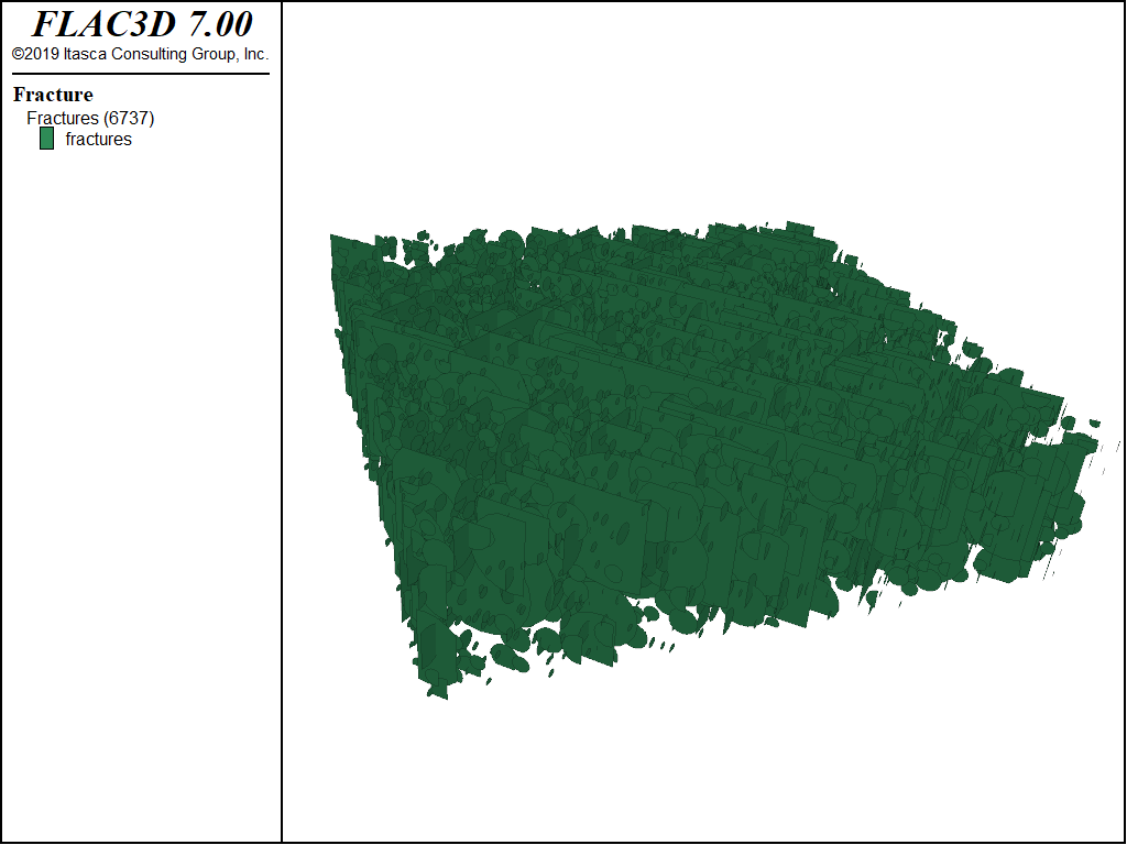
Figure 1: The Discrete Fracture Network.
Now the DFN (“fractures”) can be used to cut joints in the 3DEC model with the block cut dfn command. The resulting blocks are shown in Figure 2.
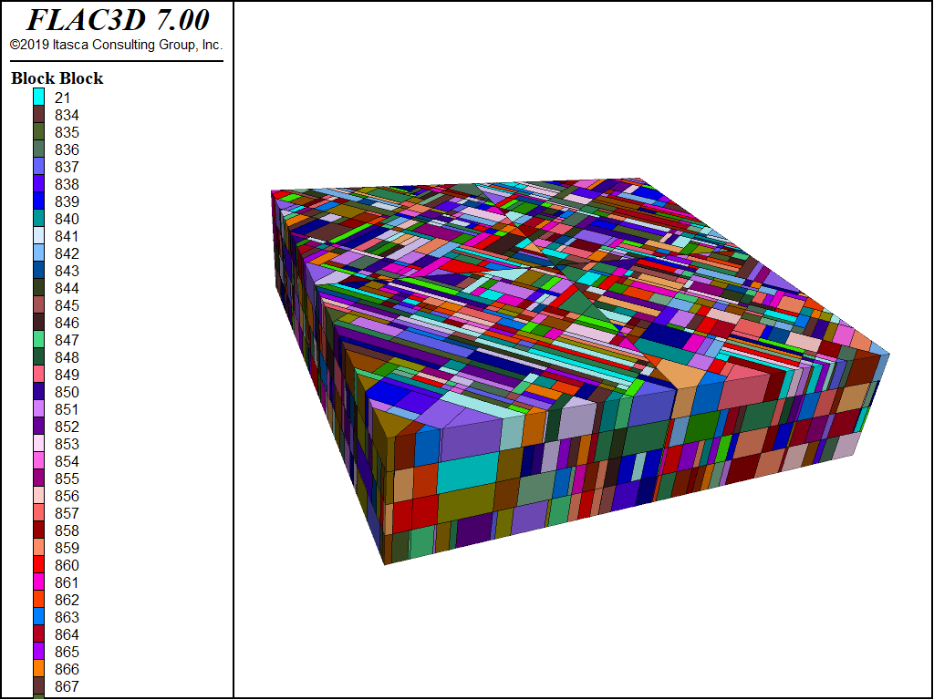
Figure 2: Blocks resulting from cutting with the DFN.
Note that the domain of the DFN is set to the outer model extents. However, the DFN is applied to the inner region because the outer region remains hidden. It is recommended that a DFN domain is set larger than the area of interest in order to eliminate any boundary issues.
The initial block model is now complete and all the blocks can be made visible. It is also good practice to save the block model prior to zoning.
Zoning
The final stage of creating the block model is to make the blocks deformable by zoning. The outer blocks are coarser while the DFN region is made finer. The edge lengths used for each range were specified as edge_size and edge_size_outer in the geometry function.
block zone generate edgelength [edge_size] range named-range 'middle'
block zone generate edgelength [edge_size_outer] range named-range 'middle' not
A record of the model information can be kept in a log file by using the following commands:
program log-file 'model_info.log'
program log on
model list info
program log off
By using the model list info command, information regarding the global variables, parameter settings, and program state information is output to the screen. Since the log file was initiated and set ‘on’, any information output to the screen is also captured and saved in the log file.
Finally, the model state is saved with the model save command. It is a good idea to also save the Project ().
Properties
A FISH function is defined for setting all the properties and assigning them to variables, similar to the geometry function defined in Step 1. The FISH code to define each property variable is as follows:
fish define set_mat_prop
  ; INPUTS
  ; Intact rock properties
  global rock_young = 20e9   ; Pa
  global rock_poisson = 0.25
  global rock_density = 2600.0
  ; Joint properties
  global joint_kn = 5.e10
  global joint_ks = 5.e10
  global joint_cohesion = 0.0
  global joint_friction = 20.0
  global joint_tension = 0.0
  global j_ap0 = 1.0e-4 ;aperture at 0 normal stress
  ; fluid properties
  global fluid_bulk_ = 3e6
  global fluid_density_ = 1000.0
  global fluid_viscosity_ = 0.0015

end
The FISH function does not assign the material properties, but simply specifies variables to store the values to be used. It is possible to simply enter the material properties directly without using FISH, however the FISH function presents a neat way to keep all parameters together and it makes it easy to change these parameters in the future.
The zones are set to be elastic and properties are assigned as shown:
block zone cmodel assign elastic
block zone property density [rock_density] young [rock_young] ...
                    poisson [rock_poisson]
Different joint properties are assigned to DFN joints, construction joints, and the hydraulic fracture plane. All joints use the Mohr-Coulomb constitutive model.
; Joints outside of the DFN
block contact jmodel assign mohr
block contact property stiffness-normal [joint_kn] stiffness-shear [joint_ks]
block contact property friction 40 cohesion 1e30 tension 1e30

; DFN joints
block contact property friction [joint_friction] cohesion [joint_cohesion] ...
  tension [joint_tension] range dfn-3dec 'fractures'

;hydrofracture plane
block contact property friction [joint_friction] cohesion [joint_cohesion] ...
  tension [joint_tension] range joint-set [hf_id]
Initial, maximum, and minimum apertures are then specified for the flow planes and fluid properties are assigned.
; flow plane properties
flowplane vertex property aperture-ini [j_ap0] aperture-min [j_ap0] ...
                          aperture-max [j_ap0]
;
; assign fluid properties
block fluid property bulk [fluid_bulk_]
block fluid property density [fluid_density_]
block fluid property viscosity [fluid_viscosity_]
In-situ stress
The in-situ stress-related variables are assigned similarly to the model and rock properties. They are defined in a FISH function and used in the commands afterwards. The parameters necessary for this example include the model depth, acceleration due to gravity, and maximum and minimum ratios of horizontal stress to vertical stress. Calculated parameters include the stresses at \(z\) = 0 and the stress gradients in the \(x\)-, \(y\)-, and \(z\)-directions, as well as the in-situ fluid pressure.
The inputs and calculations are defined in the function “set_insitu” as shown below. Then block insitu commands are executed to set the initial stresses and pore pressures.
; define insitu stress values
fish define set_insitu
  ; INPUT
  global depth = 3000.0 ; depth of model centre (m)
  global gravity_ = 9.81 ; metric,

  global kH_max=1.0 ; maximum ratio of horizontal to vertical stress (x)
  global kh_min=0.5 ; minimum ratio of horizontal to vertical stress (y)

  ; CALCULATIONS.  DO NOT CHANGE
  ; Stresses at z = 0.  Compression is negative
  global szz0 = -rock_density*depth*gravity_
  global sxx0 = kH_max*szz0
  global syy0 = kh_min*szz0

  ; fluid pressure at z = 0 (positive)
  global pp0 = fluid_density_*depth*gravity_

  ; gradients (per m in positive z direction)
  global szz_grad = rock_density*gravity_
  global syy_grad = kh_min*szz_grad
  global sxx_grad = kH_max*szz_grad
  global pp_grad = -fluid_density_*gravity_

end
[set_insitu]
;
; In-situ stress
block insitu stress [sxx0] [syy0] [szz0] 0. 0. 0. ...
             grad-z [sxx_grad] [syy_grad] [szz_grad] 0. 0. 0. nodisp

block insitu pore-pressure [pp0] gradient 0 0 [pp_grad]
Using the nodisp keyword prevents 3DEC from calculating initial normal displacements in the joints due to initial stresses. The use of “\(...\)” allows for line continuation; the two typed lines are treated as a single line of input.
Boundary Conditions
The model outer extents are fixed in place by setting the \(x\)-, \(y\)- and \(z\)-directional velocities to zero. The following commands are used to set boundary velocities:
; Boundary conditions
block gridpoint apply velocity 0 0 0 range position-x [x1_ext]
block gridpoint apply velocity 0 0 0 range position-x [x2_ext]
block gridpoint apply velocity 0 0 0 range position-y [y1_ext]
block gridpoint apply velocity 0 0 0 range position-y [y2_ext]
block gridpoint apply velocity 0 0 0 range position-z [z1_ext]
block gridpoint apply velocity 0 0 0 range position-z [z2_ext]
The maximum and minimum \(x\)-, \(y\)- and \(z\)-coordinates are used as the ranges for which the boundary condition is applied.
Solve Initial Stress State
The model is now ready to be brought to the initial stress state. Before beginning the calculation stage, we need to finalize some general model settings. Gravity is set with the model gravity command, then mechanical calculations are turned on and fluid calculations are turned off. We also set the fluid bulk modulus to zero so that pore pressures do not change as a result of mechanical deformations. A history of unbalanced force is taken. Lastly, the model is solved to equilibrium and saved.
model gravity 0 0 [-gravity_]
;
model fluid active off
model mechanical active on
block fluid property bulk 0
;
model history mechanical unbalanced-maximum
;
model solve
;
model save 'initial'
Hydraulic Fracture Simulation
After restoring the initial stress state, we begin by setting up the simulation parameters in a FISH function. We first specify the radius of the initially fractured part of the hydraulic fracture plane. A small area on this plane is “cracked” prior to injection to kick-start the fracture propagation in the rock. We then specify a maximum allowable aperture to control and maintain a reasonable time step. Finally, the injection location and injection rate are given. The locations of the various histories are also specified in the hf_setup function shown below.
model restore 'initial'
;
; define various HF parameters
fish define hf_setup

  ; INPUTS

  ; radius of initially fractured (open) part of hf
  global hf_fractured_radius = 15.0

  ; maximum allowable aperture
  global j_ap_max = 30.0e-4

  ; location of injection point
  global injection_loc = vector(0.0,0.0,0.0)

  ; volumetric injection rate
  global injection_rate = 0.05

  ; CALCULATED

  ; history locations
  global his_x = comp.x(injection_loc)
  global his_y = comp.y(injection_loc)
  global his_z = comp.z(injection_loc)
  global his_x1 = comp.x(injection_loc) - 30.0
  global his_x2 = comp.x(injection_loc) + 30.0
  global his_z1 = comp.z(injection_loc) - 30.0
  global his_z2 = comp.z(injection_loc) + 30.0
end
Next, we call a FISH file which includes several FISH functions necessary for pre-conditioning the rock mass (see hf.fis).
We begin the simulation by resetting the information regarding any recorded block and joint displacements using the block gridpoint initialize displacement command and block contact reset command. The FISH function in the “hf.fis” file called reset_aperture will do the same resetting for any recorded apertures.
Previously, the maximum joint aperture was set using the j_ap0 value. This value must be changed to allow for joint opening and fluid flow to occur. The joint property is changed with the defined maximum allowable aperture (j_ap_max) using the flowplane vertex property command.
The histories recording the time and pore pressure at the injection location and surrounding locations are specified using the following commands:
flowknot history pore-pressure position [his_x] [his_y] [his_z]
flowknot history pore-pressure position [his_x1] [his_y] [his_z]
flowknot history pore-pressure position [his_x2] [his_y] [his_z]
flowknot history pore-pressure position [his_x] [his_y] [his_z1]
flowknot history pore-pressure position [his_x] [his_y] [his_z2]
Recall that the fluid bulk modulus was previously set to zero for the initial model. We now reset the bulk modulus to the previously defined value (3 MPa) using the fluid_bulk variable. This bulk modulus is less than a true fluid; however, for the purpose of this tutorial, it will aid in speeding up the model solution with reasonable results. A minimum flow-knot volume (volmin) is also used to avoid extremely small time steps. Similarly, a minimum flowplane zone area is specified. (areamin). We also turn on the mechanical and fluid calculations to obtain a coupled solution.
block fluid property bulk [fluid_bulk_]
flowplane zone area-min 0.25
flowknot volume-min 1e-3

model fluid active on
model mechanical active on
In general, fluid time steps are larger than mechanical time steps, so many mechanical time steps may need to be executed per fluid step. The rigorous solution would solve for mechanical equilibrium after each fluid step. However, this would take a very long time, so the number of mechanical steps per fluid step may be restricted. The following command will set the maximum number of mechanical steps per fluid step to five.
model mechanical substep 5
model mechanical slave on
We now need to manually fail a small section of the hydrofracture so that the flow can get started. Subcontacts on the hydrofracture plane within a distance of hf_fractured_radius of the injection point are failed by calling a FISH function from the “hf.fis” file as shown. The crack-flow option is also turned on to restrict flow to only the failed parts of the fractures.
; Fail some part of the hydrofracture plane to permit flow
[crack_hf]
;
; flow only occurs through joints that have failed in tension
block fluid crack-flow on
Ultimately, fluid is injected into the flow knot closest to the specified location (injection_loc) with the fish function :kwd:inject.
Solution and Analysis
The calculation steps for the simulation are controlled by a FISH function that loops a certain number of times (10 in our case) and executes a command each loop iteration. In the following function, a loop index, k, is used to create the filename, fname, by associating the loop index to the saved filename after 10000 steps are executed.
To execute 3DEC commands such as model solve fluid cycles and model save within a FISH function, the FISH intrinsic command is used. After the 3DEC commands are included, end_command is used to specify the end of the 3DEC commands.
Upon executing this function ten save files will be created, each recording 10000 calculation steps. The naming convention for each file is specified by the fname variable as hf-k.sav, where k is the loop index ranging from 1 to 10.
fish define loop_solve
  loop local k (1,5)
    global fname="hf-"+string(k)
    command
model solve fluid cycles 10000
      model save [fname]
    end_command
  end_loop
end
[loop_solve]
Once the calculation is finished, plot Flow Planes, change the “Type” to “Contour” and change the “Contour” to “Joint pore pressure”. To make it easier to compare the pore pressures at the different stages, it is best to set a fixed range for the contour plot. This is done by expanding the “Contour” entry in the “Attributes” tab, expanding “Contour” again, unchecking “Auto” and setting the maximum contour to 45e6; unchecking “Auto,” and setting the minimum contour to 28e6.
The construction joints will be obscuring the area of interest. To see only the center, under the “Flow-planes joint pore pressure” plot item in the list, turn on the Clip Box, and expand it to see the area of interest. This should display a plot like this:
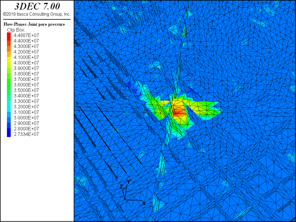
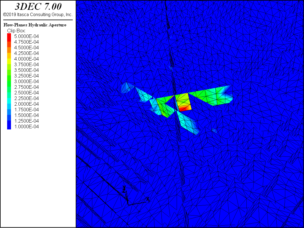
Fluid is starting to penetrate into fractures that intersect the hydraulic fracture plane. The same may be done to see the apertures:
Data Files
geometry.dat
;;-- Define geometry of hydraulic fracture model
;
model new
fish auto-create off
model large-strain off

model configure fluid
;
; Function to specify geometric parameters
fish define set_geometry

  ; INPUTS

  ; middle of model
  global xmiddle = 0.0
  global ymiddle = 0.0
  global zmiddle = 0.0

  ; size of area of interest (dfn region)
  local _modelSize_x =800
  local _modelSize_y =800
  local _modelSize_z =200

  ; hydraulic fracture joint id
  global hf_id=10000

  ; zone size in area of interest
  global edge_size=10

  ; GEOMETRY CALCULATIONS.  DO NOT CHANGE
  ; limits of area of interest (dfn region)
  global x1 = xmiddle - 0.5*_modelSize_x
  global x2 = xmiddle + 0.5*_modelSize_x
  global y1 = ymiddle - 0.5*_modelSize_y
  global y2 = ymiddle + 0.5*_modelSize_y
  global z1 = zmiddle - 0.5*_modelSize_z
  global z2 = zmiddle + 0.5*_modelSize_z

  ; limits of extended model
  global x1_ext = xmiddle - _modelSize_x
  global x2_ext = xmiddle + _modelSize_x
  global y1_ext = ymiddle - _modelSize_y
  global y2_ext = ymiddle + _modelSize_y
  global z1_ext = zmiddle - _modelSize_z
  global z2_ext = zmiddle + _modelSize_z

  ; z coordinates for extra planes
  global z_sub1 = zmiddle - 0.25*_modelSize_z
  global z_sub2 = zmiddle + 0.25*_modelSize_z

  global edge_size_outer = 3*edge_size ; outer domain discretization
end
[set_geometry]
;
; set tolerance
block tolerance 0.02
;
; create large brick
block create brick [x1_ext] [x2_ext] [y1_ext] [y2_ext] [z1_ext] [z2_ext]

;
; define inner DFN region
block cut joint-set dip 0 dip-direction 0 ori [x1] [y1] [z1]
block cut joint-set dip 0 dip-direction 0 ori [x1] [y1] [z2]
block cut joint-set dip 90 dip-direction 0 ori [x1] [y1] [z1]
block cut joint-set dip 90 dip-direction 0 ori [x1] [y2] [z1]
block cut joint-set dip 90 dip-direction 90 ori [x1] [y1] [z1]
block cut joint-set dip 90 dip-direction 90 ori [x2] [y1] [z1]

model range create 'middle' position-x [x1] [x2] ...
                            position-y [y1] [y2] position-z [z1] [z2]
block hide range named-range 'middle'
;
block densify segments 4 4 2 join
block hide off
;
block hide range named-range 'middle' not
block cut joint-set dip 90 dip-direction 0 ...
                    ori [xmiddle] [ymiddle] [zmiddle] jointset-id [hf_id]
;
block cut joint-set dip 90 dip-direction 90 ori [xmiddle] [ymiddle] [zmiddle]
block cut joint-set dip 0 dip-direction 0 ori [xmiddle] [ymiddle] [zmiddle]
block cut joint-set dip 0 dip-direction 0 ori [xmiddle] [ymiddle] [z_sub1]
block cut joint-set dip 0 dip-direction 0 ori [xmiddle] [ymiddle] [z_sub2]
;
;
; import and cut dfn
model domain extent [x1_ext] [x2_ext] [y1_ext] [y2_ext] [z1_ext] [z2_ext]
fracture import skip-errors from-file 'dfn.dat' dfn 'fractures'
;
block cut dfn id 1
;
block hide off
;
model save 'blocks'
;
; generate zones
block zone generate edgelength [edge_size] range named-range 'middle'
block zone generate edgelength [edge_size_outer] range named-range 'middle' not

;
program log-file 'model_info.log'
program log on
model list info
program log off
;
model save 'zoned'
initial.dat
; Set properties and assing initial and boundary conditions
;
model restore 'zoned'
;
; function to define material and fluid properties
fish define set_mat_prop
  ; INPUTS
  ; Intact rock properties
  global rock_young = 20e9   ; Pa
  global rock_poisson = 0.25
  global rock_density = 2600.0
  ; Joint properties
  global joint_kn = 5.e10
  global joint_ks = 5.e10
  global joint_cohesion = 0.0
  global joint_friction = 20.0
  global joint_tension = 0.0
  global j_ap0 = 1.0e-4 ;aperture at 0 normal stress
  ; fluid properties
  global fluid_bulk_ = 3e6
  global fluid_density_ = 1000.0
  global fluid_viscosity_ = 0.0015

end
[set_mat_prop]
;
; assign rock props
block zone cmodel assign elastic
block zone property density [rock_density] young [rock_young] ...
                    poisson [rock_poisson]
;
; Joint Materials - for initial stress state, maintain constant aperture
;

; Joints outside of the DFN
block contact jmodel assign mohr
block contact property stiffness-normal [joint_kn] stiffness-shear [joint_ks]
block contact property friction 40 cohesion 1e30 tension 1e30

; DFN joints
block contact property friction [joint_friction] cohesion [joint_cohesion] ...
  tension [joint_tension] range dfn-3dec 'fractures'

;hydrofracture plane
block contact property friction [joint_friction] cohesion [joint_cohesion] ...
  tension [joint_tension] range joint-set [hf_id]

; flow plane properties
flowplane vertex property aperture-ini [j_ap0] aperture-min [j_ap0] ...
                          aperture-max [j_ap0]
;
; assign fluid properties
block fluid property bulk [fluid_bulk_]
block fluid property density [fluid_density_]
block fluid property viscosity [fluid_viscosity_]
;
;
; define insitu stress values
fish define set_insitu
  ; INPUT
  global depth = 3000.0 ; depth of model centre (m)
  global gravity_ = 9.81 ; metric,

  global kH_max=1.0 ; maximum ratio of horizontal to vertical stress (x)
  global kh_min=0.5 ; minimum ratio of horizontal to vertical stress (y)

  ; CALCULATIONS.  DO NOT CHANGE
  ; Stresses at z = 0.  Compression is negative
  global szz0 = -rock_density*depth*gravity_
  global sxx0 = kH_max*szz0
  global syy0 = kh_min*szz0

  ; fluid pressure at z = 0 (positive)
  global pp0 = fluid_density_*depth*gravity_

  ; gradients (per m in positive z direction)
  global szz_grad = rock_density*gravity_
  global syy_grad = kh_min*szz_grad
  global sxx_grad = kH_max*szz_grad
  global pp_grad = -fluid_density_*gravity_

end
[set_insitu]
;
; In-situ stress
block insitu stress [sxx0] [syy0] [szz0] 0. 0. 0. ...
             grad-z [sxx_grad] [syy_grad] [szz_grad] 0. 0. 0. nodisp

block insitu pore-pressure [pp0] gradient 0 0 [pp_grad]

;
; Boundary conditions
block gridpoint apply velocity 0 0 0 range position-x [x1_ext]
block gridpoint apply velocity 0 0 0 range position-x [x2_ext]
block gridpoint apply velocity 0 0 0 range position-y [y1_ext]
block gridpoint apply velocity 0 0 0 range position-y [y2_ext]
block gridpoint apply velocity 0 0 0 range position-z [z1_ext]
block gridpoint apply velocity 0 0 0 range position-z [z2_ext]
;
model gravity 0 0 [-gravity_]
;
model fluid active off
model mechanical active on
block fluid property bulk 0
;
model history mechanical unbalanced-maximum
;
model solve
;
model save 'initial'
;
simulate.dat
; Perform the hydraulic fracture simulation
;
model restore 'initial'
;
; define various HF parameters
fish define hf_setup

  ; INPUTS

  ; radius of initially fractured (open) part of hf
  global hf_fractured_radius = 15.0

  ; maximum allowable aperture
  global j_ap_max = 30.0e-4

  ; location of injection point
  global injection_loc = vector(0.0,0.0,0.0)

  ; volumetric injection rate
  global injection_rate = 0.05

  ; CALCULATED

  ; history locations
  global his_x = comp.x(injection_loc)
  global his_y = comp.y(injection_loc)
  global his_z = comp.z(injection_loc)
  global his_x1 = comp.x(injection_loc) - 30.0
  global his_x2 = comp.x(injection_loc) + 30.0
  global his_z1 = comp.z(injection_loc) - 30.0
  global his_z2 = comp.z(injection_loc) + 30.0
end
[hf_setup]
;
; functions to support hf simulation
program call 'hf.fis'
;
; reset displacements, apertures and time
block gridpoint initialize displacement 0 0 0
block contact reset displacement
[reset_aperture]
model mechanical time-total 0
;
; change joint material to allow for joint opening
flowplane vertex property aperture-maximum [j_ap_max] range joint-set [hf_id]
flowplane vertex property aperture-maximum [j_ap_max] range dfn-3dec 'fractures'
;
;
; setup histories
flowknot history pore-pressure position [his_x] [his_y] [his_z]
flowknot history pore-pressure position [his_x1] [his_y] [his_z]
flowknot history pore-pressure position [his_x2] [his_y] [his_z]
flowknot history pore-pressure position [his_x] [his_y] [his_z1]
flowknot history pore-pressure position [his_x] [his_y] [his_z2]
;
; setup general fluid properties
block fluid property bulk [fluid_bulk_]
flowplane zone area-min 0.25
flowknot volume-min 1e-3

model fluid active on
model mechanical active on
;
; maximum number of mechanical steps per fluid step
model mechanical substep 5
model mechanical slave on
;
; Fail some part of the hydrofracture plane to permit flow
[crack_hf]
;
; flow only occurs through joints that have failed in tension
block fluid crack-flow on
;
; inject
[inject]
;
fish define loop_solve
  loop local k (1,5)
    global fname="hf-"+string(k)
    command
model solve fluid cycles 10000
      model save [fname]
    end_command
  end_loop
end
[loop_solve]
;
hf.fis
;
; Function to set small portion of hf to 'failed'
;
; INPUT: hf_fractured_radius - radius of fractured part of hf (flt)
;        injection_loc       - location of injection (v3)
;        hf_id               - id of hydrofracture joint (int)
;
fish define crack_hf
    loop foreach local cxi block.subcontact.list

        ; check if we are within given radius of borehole injection point
        local dist_ = math.mag(injection_loc - block.subcontact.pos(cxi))
        if dist_ <= hf_fractured_radius then
          block.subcontact.state(cxi) = 3 ; set state to 'tensile failure'
          block.subcontact.extra(cxi) = 3 ; for plotting
        else
          block.subcontact.state(cxi) = 0 ; set to unfailed
          block.subcontact.extra(cxi) = 0
        endif
  end_loop
end
;
; function to set mechanical aperture to initial values
;
; INPUT: j_ap0 - initial aperture (flt)
;
fish define reset_aperture
    loop foreach local fpx flowplane.vertex.list
        flowplane.vertex.aperture.mech(fpx) = j_ap0
    end_loop
end
;
;
; Function to apply injection
;
; INPUT: injection_loc - location of injection (v3)
;        injection_rate - volumetric (??) rate of injection
;
fish define inject
  local fk = flowknot.near(comp.x(injection_loc), ...
                           comp.y(injection_loc), ...
                           comp.z(injection_loc))
  flowknot.flux.fluid.app(fk) = injection_rate

  ; record history here
  global fk_x_ = flowknot.pos.x(fk)
  global fk_y_ = flowknot.pos.y(fk)
  global fk_z_ = flowknot.pos.z(fk)
  command
    flowknot history pore-pressure position [fk_x_] [fk_y_] [fk_z_]
  end_command
end
Endnotes
| [1] | To view this project and all associated data files in 3DEC, use the program menu.
⮡ 3DEC |
| Was this helpful? ... | FLAC3D © 2019, Itasca | Updated: Feb 25, 2024 |