Recording Peak Particle Velocity
In this tutorial, a dynamic wave propagation model is run and the peak particle velocity (PPV) of each gridpoint is recorded. PPV is defined as the maximum vector magnitude of velocity experienced at each point in a model.
In contrast to the previous examples, the model is driven from a FLAC3D datafile and Python is used to extend the model behavior. A Python callback function is invoked during the FLAC3D mechanical cycling and the PPV of each gridpoint is updated.
By default, no Python data is stored in the FLAC3D save files. In this
case, the save, restore and new Python callback events are
used to save and restore the PPV data to and from the FLAC3D save file.
A cube of elastic material 100 meters on a side is created. A region in the center of the cube is removed. An isotropic stress is applied to a single zone in the model to create a source of stress waves.
This model is run by evaluating the ppv.f3dat datafile.
python-reset-state false
model new
call 'ppv.py'
model config dynamic
zone create brick size 100 100 100
zone delete range position-x 40 50 position-y 40 50 position-z 40 60
zone cmodel assign elastic
zone property density 2950 young 12e9 poisson 0.25
zone dynamic damping rayleigh 0.05 150

zone face apply quiet-normal range position-x 0 position-x 100 ...
                             position-y 0 position-y 100 position-z 0 union
zone face apply quiet-strike range position-x 0 position-x 100 ...
                             position-y 0 position-y 100 position-z 0 union
zone face apply quiet-dip    range position-x 0 position-x 100 ...
                             position-y 0 position-y 100 position-z 0 union

zone initialize stress xx 10e6 yy 10e6 zz 10e6 ...
                range position-x 80 81 position-y 80 81 position-z 80 81
model solve time-total 0.08
model save "after_loading"
This data file calls ppv.py, which is shown below.
import itasca as it
it.command('python-reset-state false')
import numpy as np
np.set_printoptions(threshold=20)
from itasca import gridpointarray as gpa

ppv = None

def store_ppv(*args):
    global ppv
    if ppv is None:
        ppv = np.zeros(it.gridpoint.count())
    ppv = np.maximum(np.linalg.norm(gpa.vel(), axis=1), ppv)

def ppv_save(*args):
    global ppv
    print("saving PPV")
    if ppv.any():
        gpa.set_extra(1,ppv)

def ppv_restore(*args):
    global ppv
    print("restoring PPV")
    try:
        print(it.zone.count())
        ppv = gpa.extra(1)
        print("max ppv during restore", ppv.max())
    except: pass

def ppv_new(*args):
    global ppv
    print("resetting PPV")
    ppv = None

def transit_time():
    z = it.zone.find(1)
    K, G, rho = z.prop("bulk"), z.prop("shear"), z.density()
    vp = np.sqrt((K + 4.0/3.0*G)/rho)
    d = np.sqrt(3*100**2)
    return d/vp

it.set_callback("store_ppv", 0.1)
it.set_callback("ppv_save", "save")
it.set_callback("ppv_restore", "restore")
it.set_callback("ppv_new", "new")
The Python function store_ppv is called during each mechanical
cycle. This function uses the gridpointarray module module to get the velocity of each
gridpoint as a numpy array. The velocity magnitude of each
gridpoint is found and the maximum velocity magnitude experienced at each gridpoint is stored in the array ppv.
Saving and Restoring Python Data in FLAC3D Save Files
When the FLAC3D model is saved the Python function ppv_save is
called. In this function the PPV is stored in a gridpoint extra
variable which is then saved in the FLAC3D save file. Python functions
defined to be called during the “save” callback event are called just
before the save operation begins. Similarly, the Python function
ppv_restore is called after a FLAC3D restore operation is
completed. In this function the Python variable ppv is repopulated
with PPV values which had been stored in the gridpoint extra
variables.
When the FLAC3D model is reset from a mode new or model restore command the Python function ppv_new is called. In this
case the value of the ppv Python variable is reset.
Note
It is also possible to save and restore the value of Python variables using the it.fish functions. Values stored as FISH variables will be written to and read from the FLAC3D save file. Most common Python values can be converted into FISH values.
Data analysis using numpy and matplotlib
load_point = (80.5, 80.5, 80.5)
# distance from the source zone to each gridpoint
distance = np.linalg.norm(gpa.pos()-load_point,axis=1)

gpos = gpa.pos()
gx, gy, gz = gpos.T
top_mask = gz == 100.0
exterior_mask = reduce(np.logical_or,
                       (gx==0, gz==100, gy==0, gy==100, gz==0, gz==100))
boundary_gridpoint_mask = np.array([len(v)!=8 for v in gpa.zones()])
excavation_surface_mask = np.logical_and(np.logical_not(exterior_mask),
                                         boundary_gridpoint_mask)
interior_mask = np.logical_not(boundary_gridpoint_mask)

colors = ["#4e79a7", "#f28e2b","#e15759","#76b7b2","#59a14e",
          "#edc949","#b07aa2","#ff9da7","#9c755f","#bab0ac"]

import pylab as plt
plt.loglog(distance[interior_mask], ppv[interior_mask],
           "o", color=colors[2], markeredgewidth=0)
plt.loglog(distance[excavation_surface_mask], ppv[excavation_surface_mask],
           "o", color=colors[1], markeredgewidth=0)
plt.loglog(distance[top_mask], ppv[top_mask],
           "o", color=colors[0], markeredgewidth=0)
plt.legend(("Interior", "Excavation Surface", "Ground Surface"))
plt.xlabel("Distance from Source [m]")
plt.ylabel("PPV [m/s]")
plt.show()
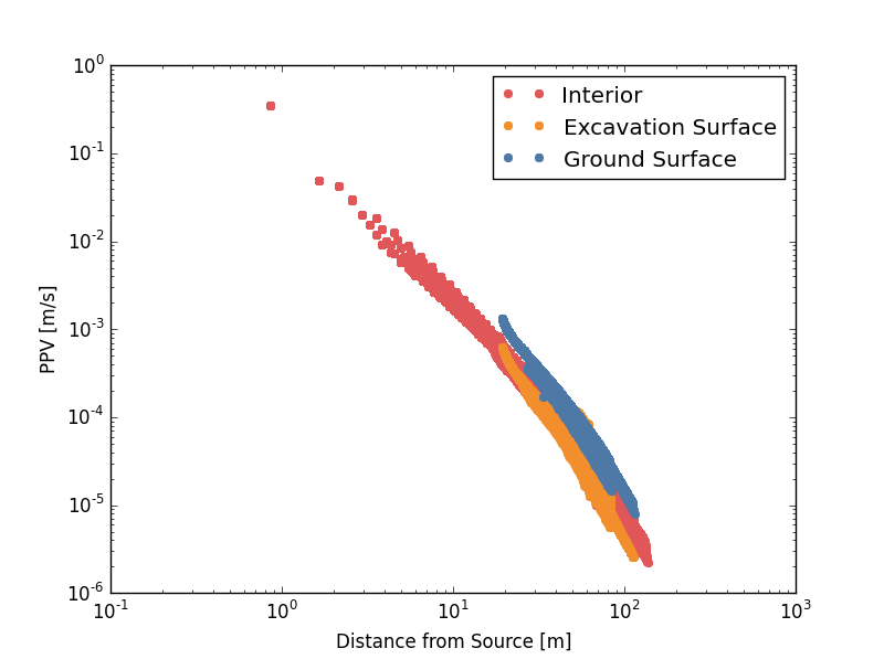
The peak particle velocity is plotted as a function of distance from the source. The data is plotted in three populations. The blue points correspond to the ground surface, the orange points correspond to the surface of the excavation and the red points correspond to the interior of the model.
Example File
The source code for this example is ppv.py
| Was this helpful? ... | FLAC3D © 2019, Itasca | Updated: Feb 25, 2024 |