Shaking Table Test with Finn Model: Simulation of the Liquefaction of a Layer
Note
To view this project in FLAC3D, use the menu command . Choose “Dynamic/ShakingTableTest” and select “ShakingTableTest.prj” to load. The main data files used are shown at the end of this example. The remaining data files can be found in the project.
The material constants in the Finn model that control pore pressure build-up are related to the volumetric response in a drained test. However, if results are available for an undrained test, then the test itself may be modeled, and the material constants deduced by comparing the numerical results with the experimental observations. Some adjustment will be necessary before a match is found.
In the following example, a “shaking table” is modeled with FLAC3D.
In this simple example, a “shaking table” is modeled with FLAC3D —this consists of a box of sand that is given a periodic motion at its base. The motion of the sides follows that of the base, except that the amplitude diminishes to zero at the top (i.e., the motion is that of simple shear). Vertical loading is by gravity only. Equilibrium stresses and pore pressures are installed in the soil, and pore pressure and effective stress (mean total stress minus the pore pressure) are monitored in a zone within the soil. A column of only one zone-width is modeled, since the horizontal variation is of no particular interest here.
The test is run for both the Martin et al. (1975) formula and the Byrne (1991) formula. The Byrne parameters correspond to \({(N_1)_{60}}\) = 6, which was selected to produce results that match those based on the given Martin parameters.
The results based on the Martin formula are shown in Figure 1, and those based on the Byrne formula are shown in Figure 2. The figures indicate similar behavior using either formula. Both show how the pore pressure at location (25, 25, 2.5) builds up with time. The history of effective stress in the same zone is also shown. It can be seen that the effective stress reaches zero after about 15 cycles of shaking (2 seconds at 5 Hz). At this point, liquefaction can be said to occur. This test is strain-controlled in the shear direction. For a stress-controlled test, collapse would occur earlier, since strain cycles would start to increase in amplitude, thus generating more pore pressure.
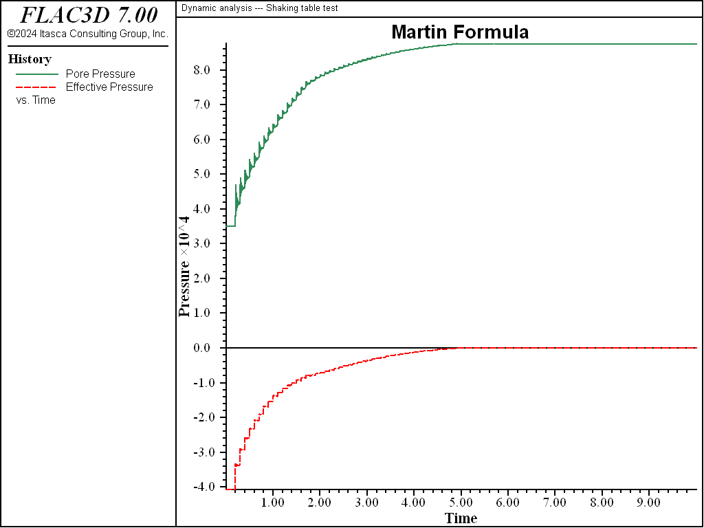
Figure 1: Pore pressure (top) and effective stress (bottom) for shaking table, using Martin.
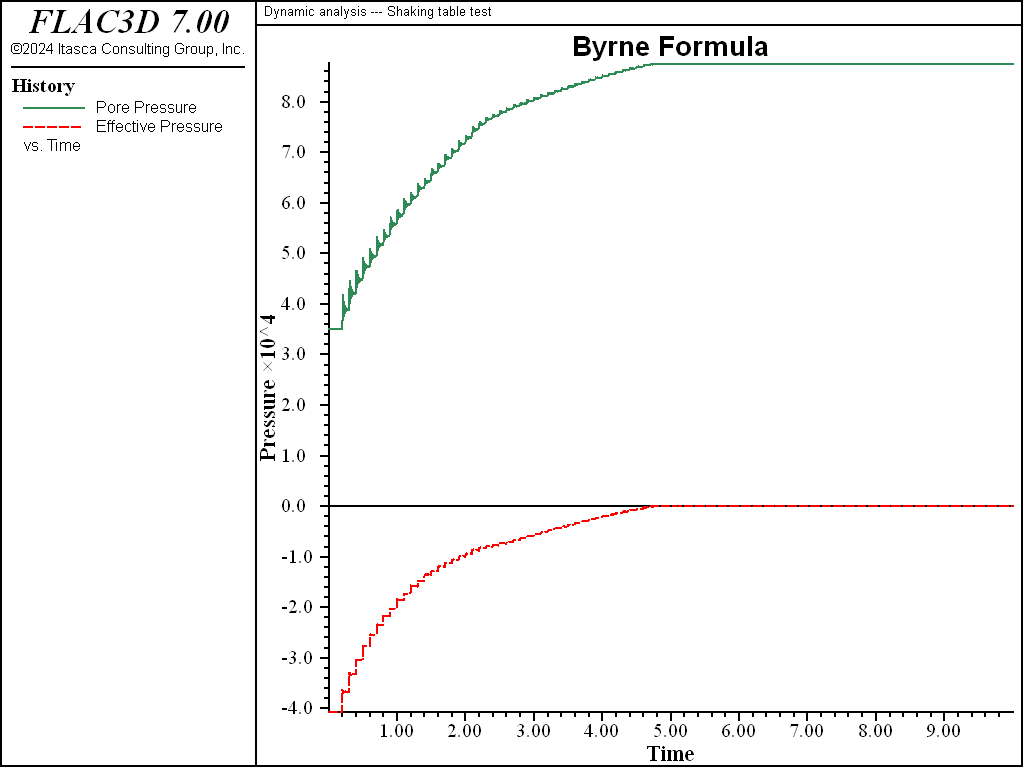
Figure 2: Pore pressure (top) and effective stress (bottom) for shaking table, using Byrne.
References
Byrne, P. “A Cyclic Shear-Volume Coupling and Pore-Pressure Model for Sand,” in Proceedings: Second International Conference on Recent Advances in Geotechnical Earthquake Engineering and Soil Dynamics (St. Louis, Missouri, March, 1991), Paper No. 1.24, 47-55 (1991).
Martin, G. R., W. D. L. Finn and H. B. Seed. “Fundamentals of Liquefaction Under Cyclic Loading,” J. Geotech., Div. ASCE, 101(GT5), 423-438 (1975).
Data File
ShakingTableTest.dat
;------------------------------------------------------------
;       Script file for dynamic problem
;       Shaking table test
;------------------------------------------------------------
model new
model large-strain off
fish automatic-create off
model title "Dynamic analysis --- Shaking table test"
model config dynamic fluid
;
; Create zones
;     Martin grid
zone create brick size 1,5,1 point 1 (50,0,0) point 2 (0,5,0) ...
                             point 3 (0,0,5) group 'Martin'
;     Byrne grid
zone create brick size 1,5,1 point 0 (0,0,10) point 1 (50,0,10) ...
                             point 2 (0,5,10) point 3 (0,0,15) group 'Byrne'
;
; Assign material model and properties
zone cmodel finn
zone fluid cmodel assign isotropic
zone property density 2000 shear 2e8 bulk 3e8 friction 35 number-latency=50
;     Parameters for Martin formula
zone property flag-switch=0 constant-1=0.80 constant-2=0.795 ...
              constant-3=0.45 constant-4=0.73 range group 'Martin'
;     Parameters for Byrne formula
fish define c1(n1_60)
    c1 = 8.7*math.exp(-1.25*math.ln(n1_60))
end
zone property flag-switch=1 constant-1=[0.5*c1(6)] constant-2=[0.4/c1(6)] ...
              constant-3=0.0 range group 'Byrne'
zone fluid property porosity 0.5
zone gridpoint initialize fluid-modulus 2e9
zone initialize fluid-density 1000
;
; Boundary Conditions
fish define sineWave(gp,dum)
    local v = 0.005 * math.sin(2 * math.pi * 5 * zone.dynamic.time.total)
    sineWave = v * (5 - gp.pos.y(gp)) / 5.0
end
zone face apply velocity-x 1 fish-local sineWave ; Apply to all faces
zone face apply velocity-normal 0 range position-y 0
zone gridpoint fix velocity-z
;
; Initial Conditions
model gravity (0,-10,0)
zone gridpoint initialize pore-pressure 5e4 gradient (0,-1e4,0)
zone initialize-stresses ratio 0.8 total
;
; Dynamic setup
zone dynamic damping rayleigh 0.05 20.0
model dynamic timestep fix 1e-4
;
; Histories
history interval 20
model history name='time' dynamic time-total
zone history name='ppm' pore-pressure position (25,1.5, 2.5)
zone history name='ppb' pore-pressure position (25,1.5,12.5)
zone history name='esm' stress-effective quantity mean position (25,1.5, 2.5)
zone history name='esb' stress-effective quantity mean position (25,1.5,12.5)
zone history velocity-x position (0,5,0)
model save 'initial'
;
; Solve to time 10 and save
model fluid active off
model solve time-total 10.0
model save 'ShakingTableTest'
| Was this helpful? ... | FLAC3D © 2019, Itasca | Updated: Feb 25, 2024 |