Geogrid Pull-out Test

Problem Statement

Note

To view this project in FLAC3D, use the menu command Help ► Examples…. Choose “Structure/Geogrid/PullOutTest” and select “PullOutTest.prj” to load. The main data files used are shown at the end of this example. The remaining data files can be found in the project.

A geosynthetic sheet is embedded in a box of soil and then pulled out of the soil, as shown in Figure 1. The total pull-out force and displacement are monitored and plotted. The test is performed for different values of confining stress. This example provides guidance in selecting geogrid properties, and demonstrates the shear response of the geogrid-soil system. It makes use of properties described in Beneito and Gotteland (2001).

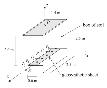
Figure 1: Geogrid pull-out test configuration.

It is assumed that both the soil (\(E\) = 15 MPa, \(\nu\) = 0.3, \(\rho\) = 1950 kg/m³) and the geogrid (\(E\) = 26 GPa, \(\nu\) = 0.33, \(t\) = 5 mm) remain elastic, and that all failure occurs at the geogrid-soil interface. The interface properties (\(k\), \(c\), \(\phi\)) are estimated as follows.

It is assumed that a set of pull-out tests have been performed at different confining pressures. The value of \(k\) is set equal to the slope of the pull-out stress versus displacement plot. In Beneito and Gotteland (2001), this slope increases for increasing confinement. For our purposes, the slope for a confinement of 39 kPa (which corresponds with the weight of the soil above the geogrid) is matched by setting

(1)\[k = {\Delta S \over \Delta U} = {23\hbox{ kPa} \over 10\hbox{ mm}} = 2.3\times10^6\hbox{ N/m$^3$}\]

where:	\(S\)	= pull-out stress (pull-out force/(embedded geogrid area)); and
	\(U\)	= pull-out displacement.

The values of \(c\) and \(\phi\) are found from a plot of maximum pull-out force versus confinement. The slope of this curve equals \(\tan\phi\), and the \(y\)-intercept equals \(c\). In Beneito and Gotteland (2001), the cohesion is zero, and the maximum pull-out stress for confinements of 100 and 25 kPa is 54 and 12 kPa, respectively. For our purposes, these data are matched by setting

(2)\[\begin{split}\begin{split} c &= 0 \\ \phi &= \tan^{-1}\left( {54 - 12 \over 100 - 25} \right) = 29.2\hbox{ degrees} \end{split}\end{split}\]

The FLAC3D model consists of 60 geogrid elements and 250 zones, as shown in Figure 2. The grid is customized for the test using the Extruder tool, and the data file is exported from the State pane. The modeling sequence then proceeds as follows. Begin with a stress-free soil, fix the sides and bottom of the box, install the geogrid, activate gravity, apply a constant pressure to the top surface (in the initial run, this pressure is zero) and use the zone initialize-stresses command to reach equilibrium. At this stage, the sides and bottom of the box are being compressed by the soil, and a confining stress of 39 kPa is acting on the geogrid surface.

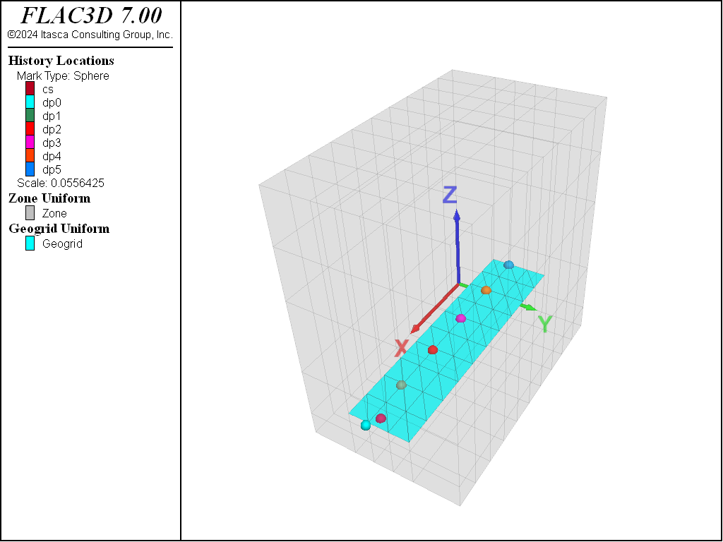
Figure 2: FLAC3D model for geogrid pull-out test.

The pull-out test is performed by applying a constant horizontal velocity to the geogrid nodes along the box front. These nodal velocities are fixed in the geogrid plane (which corresponds with the node-local \(xy\)-axes — see the structure node initialize command), and then specify a velocity in the global \(x\)-direction. During the test, the applied displacement and force are monitored. The applied force is equal to the total out-of-balance force acting on the geogrid nodes along the box front (computed with the pullOutStress FISH function), and the pull-out stress equals this force divided by the embedded geogrid area. Also monitored is the total shear displacement in the six coupling springs along the geogrid centerline at 0.5 m intervals from front to back, and the coupling stress in the front node. (The locations of the history monitoring points are shown in Figure 2).

The pull-out stress versus applied displacement is shown in Figure 3 for the case in which no pressure is applied to the top surface. An applied displacement of approximately 10 mm is necessary to mobilize all of the frictional resistance of the geogrid. During this test, the effective confining stress acting on the geogrid surface is equal to 39 kPa. For this value of confinement, and for the geogrid interface properties specified, the maximum shear stress should equal 21.8 kPa. The value obtained is 21.6 kPa, which matches the theoretical value. Also, the slope of this curve equals the coupling spring stiffness (see equation (1)).

Figure 3 also compares the evolution of the shear stress acting in the coupling spring at the front face with the pull-out shear stress. It is found that the front coupling spring yields before the overall system yields. This is to be expected, because the yielded region begins at the front face and then propagates back into the soil block. Also found is that the maximum stress in the coupling spring slightly exceeds that of the overall system (22.19 kPa versus 21.6 kPa). Also, the effective confining stress acting on the coupling spring at the front face (structure geogrid list coupling range component-id 57) equals 40.03 kPa, which is slightly more than the average value of 39 kPa acting on the entire geogrid. Figure 3 illustrates the difference between the local response at a geogrid node and the global response of the entire geogrid system. In the entire system, the effective confining stress differs over different parts of the geogrid because of boundary effects from the box walls.

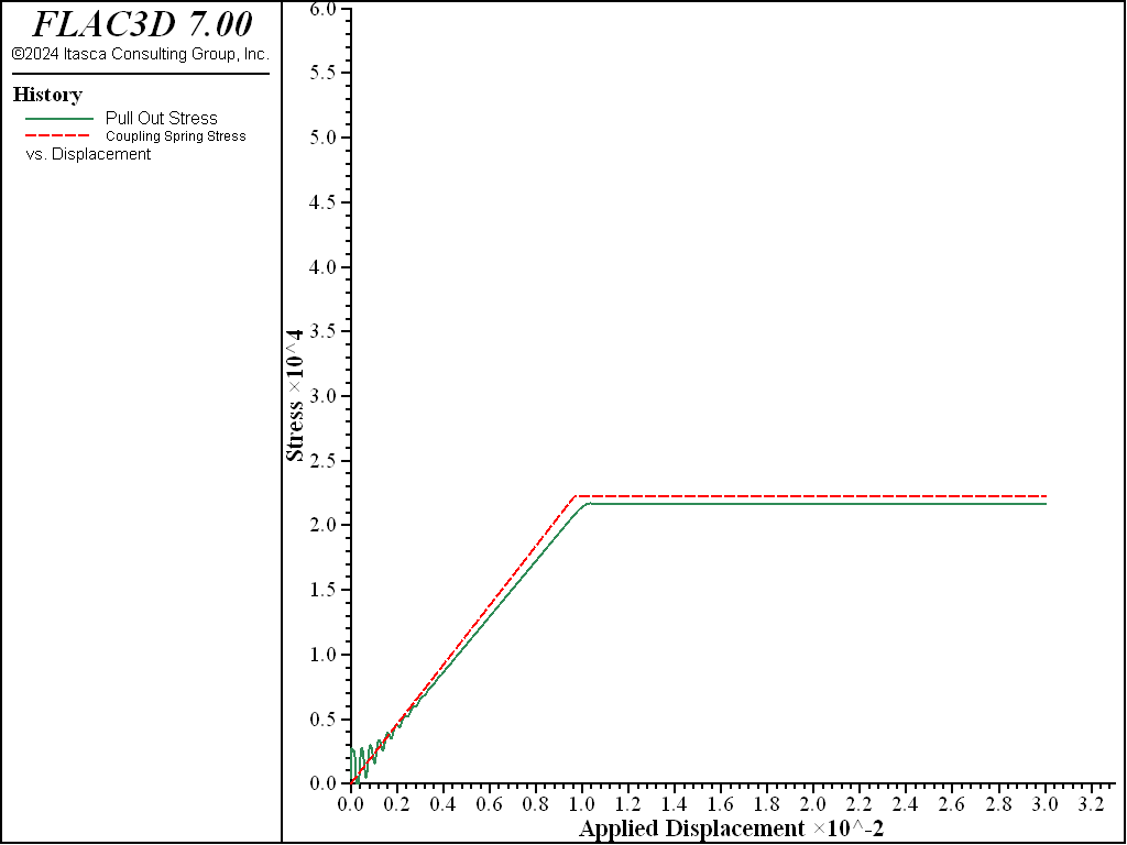
Figure 3: Pull-out shear stress and coupling spring stress at \(P_0\) versus applied displacement (no pressure applied to top surface).

In Figure 4, the geogrid displacements, \(U_i\), are plotted at the locations \(P_i\) (from Figure 1) versus the applied displacement \(U_0\) over the range from 9 to 12 mm. In this plot, the histories 10-15 correspond with the points \(P_0\)-\(P_5\), respectively. Observe the phenomenon of progressive mobilization of the geogrid as the yielded region progresses inward from the front face. The equal slopes indicate that all points are moving at the same rate as the front face, and the offsets demonstrate that the front points have moved farther than the back points (also see Figure 5). The very small offset occurs because the geogrid is much stiffer than the surrounding soil, such that very little strain develops in the geogrid itself prior to yielding.

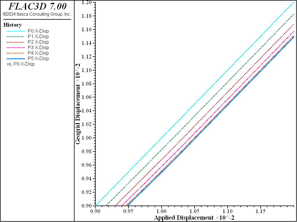
Figure 4: Displacements along geogrid centerline versus applied displacement (no pressure applied to top surface).

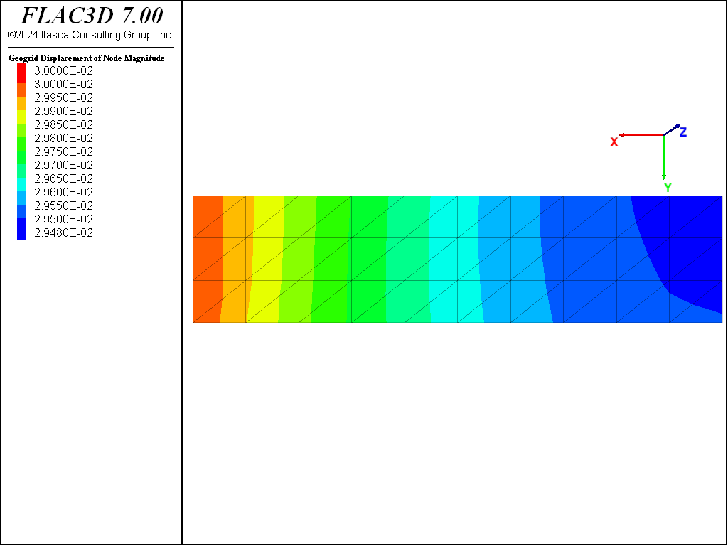
Figure 5: Geogrid displacement field (\(U_0\) = 12 mm; no pressure applied to top surface).

At an applied displacement of 30 mm, the shear stresses acting on the geogrid are examined (see Figure 6) as well as the membrane stress resultant, \(N_x\) (where the \(x\)-direction is parallel with the global \(x\)-direction), acting within the geogrid (see Figure 7). In Figure 8, the yield state of the coupling springs is overlayed. First, note that all of the coupling springs are yielding. The shear stresses acting on the geogrid have reached a constant maximum value that ranges from 21.2 to 22.2 kPa over the geogrid surface. The value is largest at the front face, and slightly lower at the far end. The membrane stress resultant acting within the geogrid is largest at the front face (53.7 kN/m), and declines as one moves away from the face. This occurs because more load is transferred to the soil as one moves away from the front face. The membrane stress is constant across the geogrid width; thus, the stress in the global \(x\)-direction at the mid-surface can be estimated by dividing the value of \(N_x\) by the geogrid thickness to yield 10.7 MPa, which is what is seen in the contour plot in Figure 8. The actual \(xx\)-stress in a geogrid element adjacent to the front face is found to be 10.01 MPa.

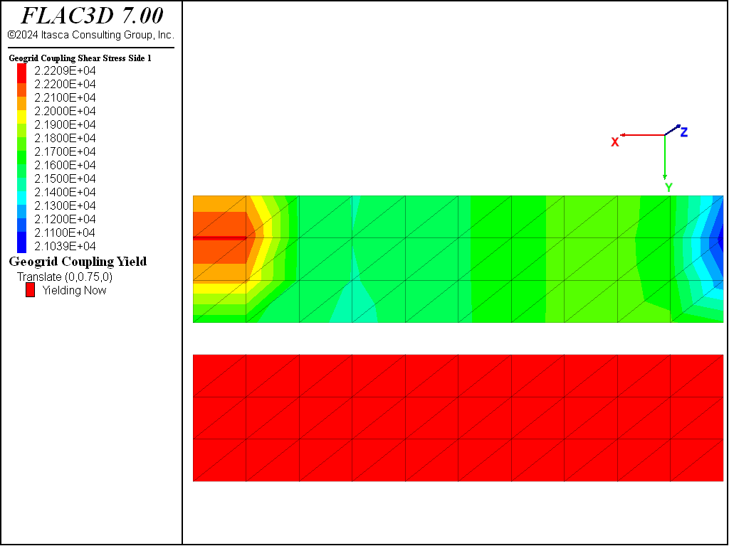
Figure 6: Shear stresses acting on the geogrid (\(U_0\) = 12 mm; no pressure applied to top surface).

Figure 7: Membrane stress resultant \(N_x\) acting within the geogrid (\(U_0\) = 12 mm; no pressure applied to top surface).

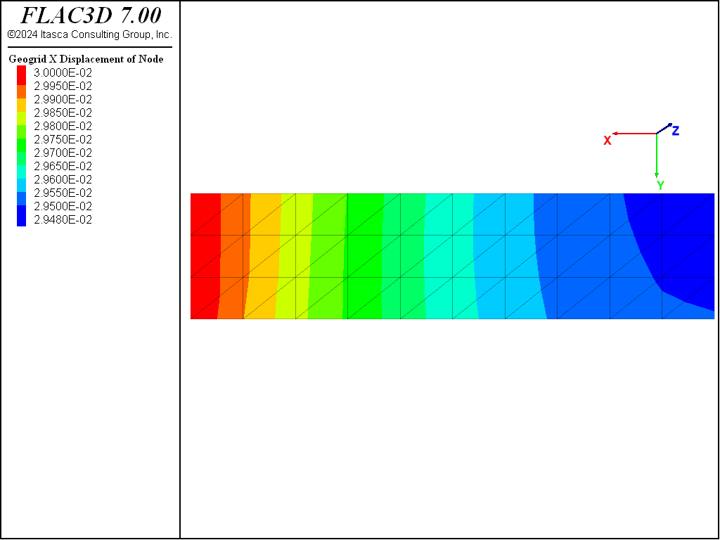
Figure 8: xx-stress acting within the geogrid (\(U_0\) = 12 mm; no pressure applied to top surface).

The simulation is rerun with an applied pressure of 61 kPa on the top surface. This increases the geogrid confinement to 100 kPa, which corresponds with the laboratory data used in equation (2), and for which the expected maximum pull-out stress is 54 kPa. The computed value equals 55.4 kPa (see Figure 9).

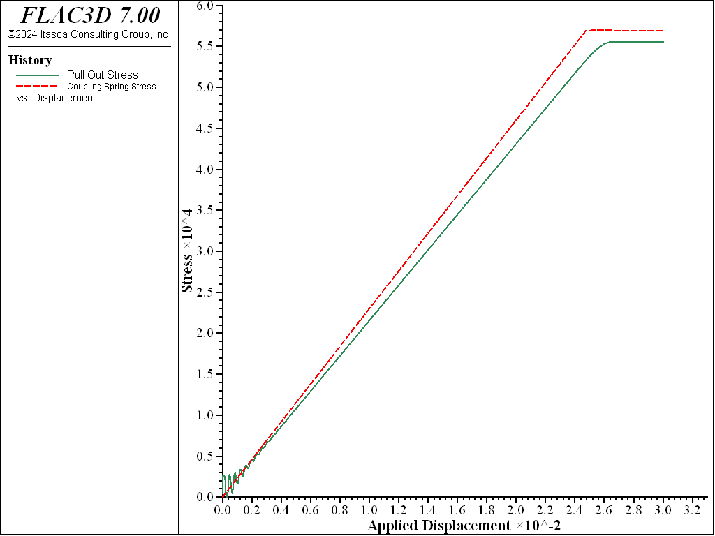
Figure 9: Pull-out shear stress versus applied displacement (pressure of 61 kPa applied to top surface).

Reference

Beneito, C. and Ph. Gotteland. “Three-Dimensional Numerical Modeling of Geosynthetics Mechanical Behavior,” in FLAC and Numerical Modeling in Geomechanics (Proceedings of the Second International FLAC Symposium on Numerical Modeling in Geomechanics, Lyon, France, 29-31 October 2001). D. Billaux et al., eds. Lisse: Balkema (2001).

Data File

PullOutTest.dat

model new
model large-strain off
model title "Geogrid Pull-Out Test"
; Zones created interactively using Extruder, exported to State Pane
program call 'geometry' suppress
zone generate from-extruder
zone face skin ; Label model boundaries
; Assign zone model and properties
zone cmodel assign elastic
zone property bulk=12.5e6 shear=5.77e6 density=1950. ; E=15 MPa, nu=0.3
; Boundary conditions
zone face apply velocity-normal 0 range group 'East' or 'West'
zone face apply velocity-normal 0 range group 'North' or 'South'
zone face apply velocity-normal 0 range group 'Bottom'
; Create the geogrid, embedded in the zone, and assign properties
struct geogrid create by-quadrilateral (0,0.45,0.5) (2.5,0.45,0.5) ...
                                       (2.5,1.05,0.5) (0,1.05,0.5) ...
                                       size (10,3)
struct geogrid property isotropic=(26e9, 0.33) thickness=5e-3 ...
                        coupling-stiffness=2.3e6 coupling-cohesion=0.0 ...
                        coupling-friction=29
; Tag nodes on front
struct node group 'Front' range position-x 2.5
; Init globals and solve
model gravity 10
zone initialize-stresses ratio 0.3
history interval 1
[global groups = struct.node.group(::struct.node.list,'Default')]
[global frontNodes = struct.node.list(groups=='Front')]
fish define pullOutStress
    return list.sum(-struct.node.force.unbal.global(::frontNodes,1)) / 1.5
end
struct node fix velocity-x range group 'Front' ; fix velocity in geogrid plane
struct node fix velocity-y range group 'Front' ;   (node-local xy-axes)
struct node initialize velocity-x 2e-6 local range group 'Front'
struct node initialize displacement (0,0,0)
struct node initialize displacement-rotational (0,0,0) ; reset nodal displ.
; Nodal displacement histories
struct node history name='dp0' displacement-x position (2.5,0.65,0.5)
struct node history name='dp1' displacement-x position (2.0,0.65,0.5)
struct node history name='dp2' displacement-x position (1.5,0.65,0.5)
struct node history name='dp3' displacement-x position (1.0,0.65,0.5)
struct node history name='dp4' displacement-x position (0.5,0.65,0.5)
struct node history name='dp5' displacement-x position (  0,0.65,0.5)
fish history name='stress' pullOutStress
struct geogrid history name='cs' coupling-stress component-id 57 node 2
; Setup model damping
struct mechanical damping combined-local
model save 'Initial'
;; ;;;;;;;;;;;;;;;;;;;;;;;;;;;;;;;;;;;;;;;;;;;;;;;;;;;;;;;;;;;;;; 
;; No pressure applied to top surface
model cycle 15000 
model save 'Pressure-0k'
;; ;;;;;;;;;;;;;;;;;;;;;;;;;;;;;;;;;;;;;;;;;;;;;;;;;;;;;;;;;;;;;; 
;; 61kPa pressure applied to top surface
model restore 'Initial'
zone face apply stress-zz -61e3 range group 'Top'
zone initialize-stresses ratio 0.3 overburden -61e3
model cycle 15000 
model save 'Pressure-61k'