Maxwell/Kelvin/Burgers Model: Parallel-Plate Viscometer

Note

To view this project in 3DEC, use the menu command Help ► Examples…. Choose “CreepMaterialModels/Viscometer” and select “Viscometer.prj” to load. The project’s main data files are shown at the end of this example.

This example is to verify the classical Maxwell model and Burgers model. Suppose that a material with viscosity \(\eta\) is steadily squeezed between two parallel plates that are moving at a constant velocity \(V_0\). The two plates have length 2 \(l\) and are a distance 2 \(h\) apart. The material is prevented from slipping at the plates. The approximate analytical solution, given by Jaeger (1969), is

\[\begin{split}\begin{split} V_x\ &=\ {{3 V_o x\ (h^2 - y^2)} \over {2 h^3}} \\ V_y\ &=\ {{V_o y (y^2 - 3 h^2)} \over {2 h^3}} \\ \sigma_{xx}\ &=\ 3 \eta V_o\ \biggl[ {{3 (h^2 - y^2) + x^2 - l^2} \over {2 h^3}} \biggr] \\ \sigma_{yy}\ &=\ 3 \eta V_o\ \biggl[ {{y^2 - h^2 + x^2 - l^2} \over {2 h^3}} \biggr] \\ \sigma_{xy}\ &=\ -3 \biggl[ {{ V_o\ \eta\ x\ y} \over {h^3}} \biggr] \end{split}\end{split}\]

The problem is illustrated in Figure 1.

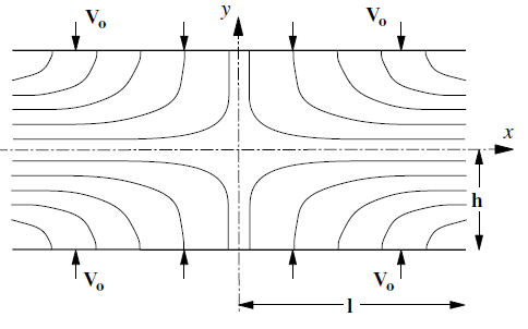
Figure 1: Parallel-plate viscometer showing velocity streamlines (Jaeger 1969).

To solve the problem with 3DEC, advantage can be taken of the symmetry about the \(x\)- and \(y\)-axes. Only the top-right quadrant needs to be modeled. For compatibility with the approximations of the analytical solution, artificial forces have to be applied at the “free” right-hand edge, and small-strain logic is used.

The material properties are

shear modulus	5 × 108 Pa
bulk modulus	1.5 × 109 Pa
viscosity	1 × 1010 kg/ms

The Maxwell model component is also tested in the Burgers-Mohr model (block zone cmodel burgers-mohr) for the viscometer test. The values of cohesion and tensile strength are set high to prevent plastic failure in the viscoplastic model so it is equivalent to the classical Burgers model. The additional commands for this model are contained in main data files. Upon execution of the data file with each model activated, results identical to those produced with the classical viscoelastic model are obtained.

The analytical solution is calculated with FISH function anal, using the extended arrays to store the calculated values. A good agreement was obtained between 3DEC and the closed-form solution. The contours of \(x\)-velocity are plotted in Figure 2. The corresponding analytical solution is shown in Figure 3.

Figure 2: Contours of \(x\)-velocity from 3DEC.

Figure 3: Contours of \(x\)-velocity from the analytical solution (from gridpoint extra array 1).

Data Files

viscometer.dat

model new
; file: viscometer.3dip-directionat
; classical viscosity - parallel plate test
;
model title
"Parallel-Plate Viscometer (Classical Viscosity)"
model configure creep
model large-strain off

block create brick 0 10 0 1 0 5
block zone generate edgelength 1.0
block zone cmodel assign maxwell
block zone property density 1 bulk 1.5e9 shear 0.5e9 viscosity 1e10

block gridpoint apply velocity-x = 0 range position-x 0
block gridpoint apply velocity-z 0 range position-z 0
block gridpoint apply velocity-x 0 range position-z 5
block gridpoint apply velocity-z -1e-4 range position-z 5
block gridpoint apply force-x 2.25e5 range position-x 10 position-z 0
block gridpoint apply force-x 4.32e5 force-z -1.2e5 ...
  range position-x 10 position-z 0.9 1.1
block gridpoint apply force-x 3.78e5 force-z -2.4e5 ...
  range position-x 10 position-z 1.9 2.1
block gridpoint apply force-x 2.88e5 force-z -3.6e5 ...
  range position-x 10 position-z 2.9 3.1
block gridpoint apply force-x 1.62e5 force-z -4.8e5 ...
  range position-x 10 position-z 3.9 4.1
block gridpoint apply velocity-y 0 range position-y 0
block gridpoint apply velocity-y 0 range position-y 1

model creep active on
model creep timestep fix 1

model history creep time-total
model history mechanical unbalanced-maximum
block history velocity-x position 3 3 0
block history velocity-y position 3 3 0
block history stress-xx position 3.5 3.5 0.5
block history stress-yy position 3.5 3.5 0.5
block history stress-xy position 3.5 3.5 0.5
block history stress-zz position 3.5 3.5 0.5

model save 'ini'

model step 500

fish define anal(vel_mag,height,length,visc_val)
;  parallel plate viscometer analytical solution
;
;    gp.extra 1 : x-velocities
;             2 : y-velocities
;    zone.extra  1 : xx-stresses
;             2 : yy-stresses
;             3 : xy-stresses

    loop foreach local p_gp block.gp.list
        local xv_top = (height^2)-(block.gp.pos.z(p_gp)^2)   
              xv_top = -3.0 * vel_mag*block.gp.pos.x(p_gp) * xv_top   
        block.gp.extra(p_gp,1) = xv_top / (2.0*(height^3.0))
;        
        local yv_top = block.gp.pos.z(p_gp)^2 - 3.0*(height^2)
              yv_top = -1.0 * vel_mag*block.gp.pos.z(p_gp) * yv_top
        block.gp.extra(p_gp,2) = yv_top / (2.0*(height^3))
    endloop
  
    loop foreach local p_z block.zone.list
      local xx_one = 3*((height^2)-(block.zone.pos.z(p_z))^2)
      local xx_two = (xx_one + (block.zone.pos.x(p_z)^2-length^2))/(2.0*(height^3))
      block.zone.extra(p_z,1) = - xx_two * 3 * visc_val * vel_mag
;  
      local yy_one = block.zone.pos.z(p_z)^2 - height^2
      yy_one = yy_one + block.zone.pos.x(p_z)^2 - length^2
      local yy_two = yy_one / (2.0*(height^3))
      block.zone.extra(p_z,2) = - yy_two * 3 * visc_val * vel_mag
;  
      local temp = 3*vel_mag*visc_val*block.zone.pos.x(p_z)*block.zone.pos.z(p_z)
      block.zone.extra(p_z,3)=temp/(height^3)
    endloop
end
[anal(-1e-4,5,10,1e10)]

model save "viscometer"