3DEC Theory and Background • Factor of Safety

Factor of Safety Contours

Problem Statement

Note

To view this project in 3DEC, use the menu command Help ► Examples…. Choose “TheoryAndBackground/FactorOfSafety/ FOS_Contours” and select “FOS_Contours.prj” to load. The project’s main data files are shown at the end of this example.

Typically, application of the strength reduction method produces one single factor of safety per simulation, corresponding to one global minimum stability state. However, the ability to calculate multiple minimum states may be of interest, for example, along a complex slope profile such as a benched cut or a slope with a berm (e.g., see Cheng et al. 2007). A “safety map” may be constructed through a series of analyses using the limit equilibrium method to identify multiple possible failure surfaces for slopes of this type (Baker and Leshchinsky 2001).

A simple procedure to determine multiple local stability states with the strength reduction method is to exclude different regions of the slope when performing the strength reduction calculation.

Alternatively, the explicit dynamic solution method employed in 3DEC allows multiple local stability surfaces to be identified in one 3DEC simulation. When using the model factor-of-safety command the velocity magnitude of each grid point is stored for each global factor of safety tested. This data is stored as part of the model state. By comparing the velocity data at a grid point against a limiting velocity you can determine the greatest factor of safety checked that resulted in that specific grid point being stable.

By using the bracket-limit keyword you can guarantee that there will be enough tests to fill out a meaningful contour map.

Finding the limiting velocity that determines if a given gridpoint should be considered stable or unstable can be done after the fact, by examining the velocities from the last unstable state and by trying different values in the factor of safety plot until a result seems acceptable.

This technique is demonstrated for a slope profile consisting of two double-inclination slopes separated by a horizontal berm. This example is taken from Cheng et al. (2007), who produced a set of local minimum stability states for this slope using the Morgenstern-Price limit equilibrium method. The slope configuration and resulting local minima locations are shown in Figure 1.

3DEC Model

The slope geometry is created by joining together bricks and prisms.

The 3DEC simulation run to determine the minimum factor of safety for this slope using the model factor-of-safety command. The result, shown by the shear strain contour plot in Figure Figure #fos_shearstrain, is a global minimum factor of safety of 1.39 with a multiple failure surface that corresponds to the two surfaces with the smallest factor of safety values shown in the lower slope in Figure 1.

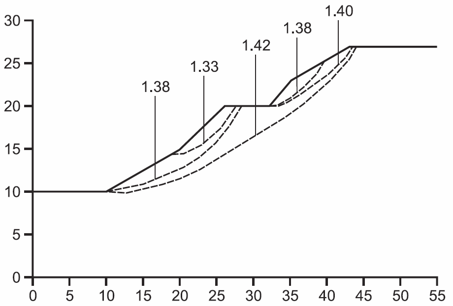
Figure 1: Local minima surfaces from limit equilibrium solution for slope with berm (from Cheng et al. 2007).

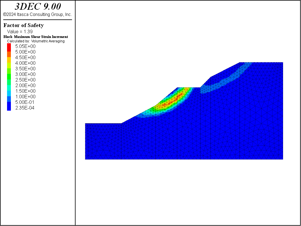
Figure 2: Global minimum factor of safety for slope with berm.

The factor of safety contour plot produced for this example is shown in Figure Figure #fos_contours. This is plotted by selecting Contours and Factor of Safety in the Block plot item, and then entering a velocity threshold of 0.01. The contours compare quite well with the local minima surfaces plot in Figure 1. Note that the global minimum contour line (at a factor of 1.25) in Figure Figure #fos_contours closely matches the smallest local minimum surface in Figure 1. The next contour lines, at factors of 1.35 and 1.4 below and above the berm, also compare well with the failure surfaces identified in Figure 1. The factor of safety contour plot also shows a contour shape (see, for example, the 1.45 contour in Figure Figure #fos_contours) that curves upward beneath the berm. Note that this effect on the shape of the failure surface is not seen with the limit equilibrium method; compare to the 1.42 surface in Figure 1.

This exercise demonstrates that the strength reduction method can be applied to produce multiple potential failure surfaces in one simulation by monitoring failure in terms of the development of unstable regions (defined by high gridpoint velocities) as the strength of the material is incrementally reduced.

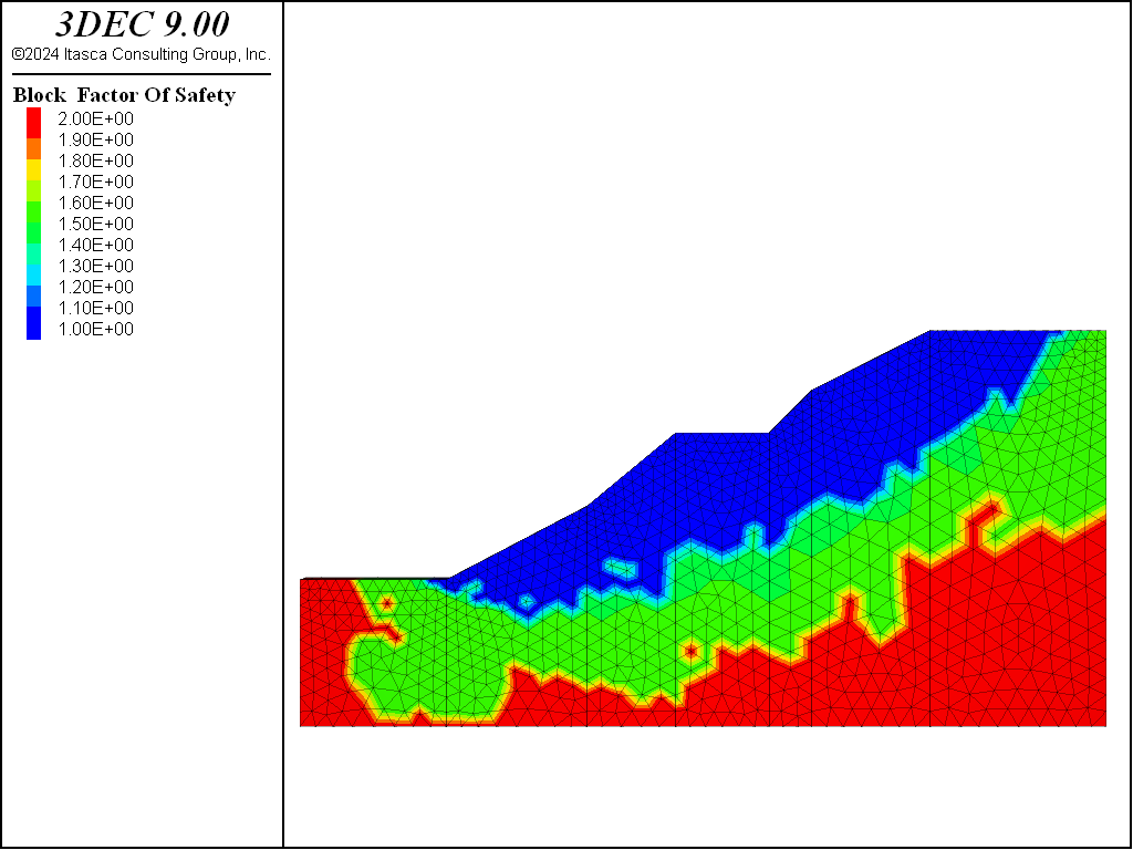
Figure 3: Factor of safety contours for slope with berm.

References

Baker, R., and D. Leshchinsky. “Spatial distribution of safety factors,” J. Geotech. Geoenviron. Eng., 127(2), 135-45 (2001).

Cheng, Y.M., T. Lansivaara and W.B. Wei. “Two-dimensional slope stability analysis by limit equilibrium and strength reduction methods,” Computers and Geotechnics, 34, 137-150, 2007.

Data Files

slope_FOS.dat

model new
model random 10000
model large-strain off

block create brick 0 10 0 1 0 10
block create brick 43 55 0 1 0 27
block create brick 25.6 32 0 1 0 20
block create prism face-1 34.92,0,0 43,0,0 43,0,27 34.92,0,22.92 ...
                   face-2 34.92,1,0 43,1,0 43,1,27 34.92,1,22.92
block create prism face-1 32,0,0 34.92,0,0 34.92,0,22.92 32,0,20 ...
                   face-2 32,1,0 34.92,1,0 34.92,1,22.92 32,1,20
block create prism face-1 19.559,0,0 25.6,0,0 25.6,0,20 19.559,0,15 ...
                   face-2 19.559,1,0 25.6,1,0 25.6,1,20 19.559,1,15
block create prism face-1 10,0,0 19.559,0,0 19.559,0,15 10,0,10 ...
                   face-2 10,1,0 19.559,1,0 19.559,1,15 10,1,10
                   
block join

; smaller zones on the edges
block zone size edgelength 0.5 range position-z 10 27 by block-gridpoint
block zone generate-new minimum-edge 0.5 maximum-edge 2

block zone cmodel assign mohr-coulomb
block zone property bulk 6.25e6 shear 2.88462e6 density 2000
block zone property cohesion 5000 friction 30 tension 1e100

block gridpoint apply velocity 0 0 0 range position-z 0
block gridpoint apply velocity-x 0.0 range position-x 0 
block gridpoint apply velocity-x 0.0 range position-x 55 
block gridpoint apply velocity-y 0.0 range position-y 0 
block gridpoint apply velocity-y 0.0 range position-y 1

model gravity 10
block zone nodal-mixed-discretization on
model solve elastic ratio 1e-6
model save 'equil.sav'

block gridpoint initialize velocity 0 0 0
block gridpoint initialize displacement 0 0 0
model factor-of-safety