Open Pit with Octree Blocking
Problem Statement
Note
The project file for this example may be viewed/run in 3DEC.[1] The data files used are shown at the end of this example.
This example will describe the basic commands used to import geometry sets and create a 3DEC model of an open pit mine. This tutorial involves the use of predefined geometries created from contour lines. The geometries used are stereo lithography (*.stl) file types which 3DEC is capable of importing (assuming that they are joined shapes). The three *.stl files included in this tutorial are “pit.stl,” “ore.stl,” and “tunnel.stl.” 3DEC can also import AutoCAD document exchange format (dxf) files in the same way.
3DEC Model Geometry
The model is constructed by starting with one large block and cutting it into smaller blocks to define the pit geometry. The block create brick command is used and x, y and z limits are provided. This model uses the Imperial system of units and therefore the block coordinates are in feet. Before creating the first block, a general model tolerance is specified using the block tolerance command. The default tolerance setting is 0.0012 × the average model dimensions in x, y, and z. For this example, the default is too large and thus we require a smaller value.
Next, the initial brick is cut into smaller blocks (6x6x3). This will improve the resolution of model geometry and will also speed up the zone generation. This could be done with a series of block cut commands but it is simpler to use the block densify command.
The joints created with the command are not geological joints, but are simply used in defining geometry. Therefore the join keyword is used to join the blocks across the joints. The blocks at this point are shown in Figure 1
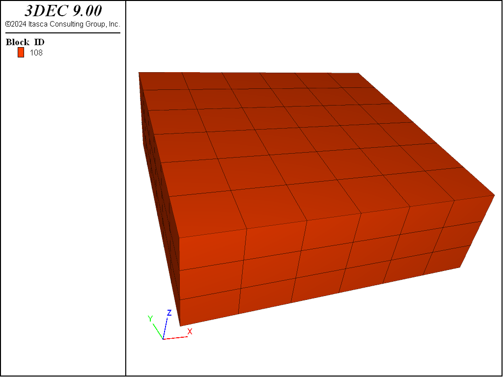
Figure 1: Initial blocks making up the open pit model
Geometries
Now that the block model has been created, we can now import the predefined geometries. First, copy the *.stl files to your project’s folder. The *.stl files are found in the “DataFiles3D3DECExampleApplicationsOctree_pit” folder located where the program was installed. Import the geometries using geometry import commands.
Alternatively, you could import the files by going to File → Open Item, but be aware that if you re-execute the data file “pit_zoned.3ddat” (as you are about to), the geometries will not be imported because using the File menu will not create the necessary commands in the data file.
The imported geometries can now be plotted by adding the Geometry plot item under User Defined Data. Ensure that both sets are checked under Imported Sets in the Plot Item Attributes. The geometries are shown in Figure 2.
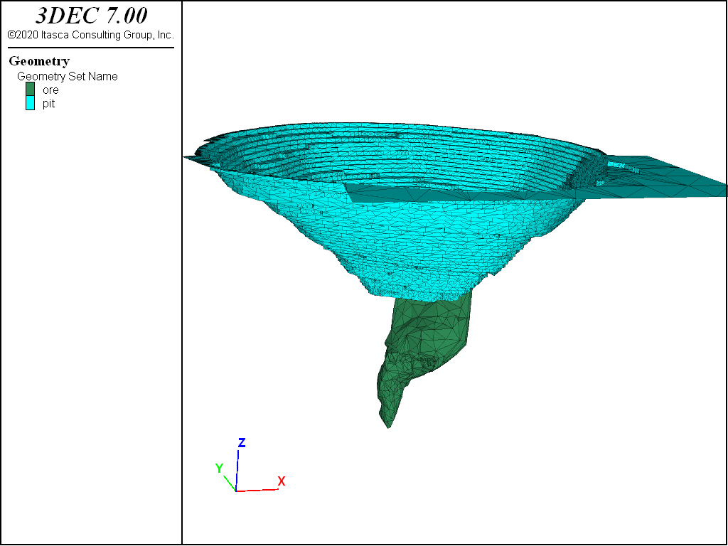
Figure 2: Imported pit and ore geometries.
The block densify command is now used again to create a higher resolution block model for simulations. The densify block command with the repeat keyword and range geometry will automatically cuts blocks close to the geometries and develops an octree mesh. Octree meshes are based on an increasingly finer decomposition of space into hexahedral blocks. In this case, the range is the pit and ore geometry.
The operation iteratively finds blocks that are touching the geometry (dist 0 extent) and splits them into 8 blocks. The operation is repeated 4 times to ensure the blocks in the area of interest are small enough to define the pit and ore geometry. The gradlimit keyword ensures that adjacent blocks are not more than one level of densification different (i.e., it ensures there are not very big blocks next to very small blocks). Blocks are joined using the join keyword. See the block densify for further information.
Next, we introduce a geological fault with a dip of 60^{circ}, dip direction of 250^{circ}, and origin of (14200, -24300, -270) placing the fault outside of the pit dipping towards it. The model at this point is shown in Figure 3.
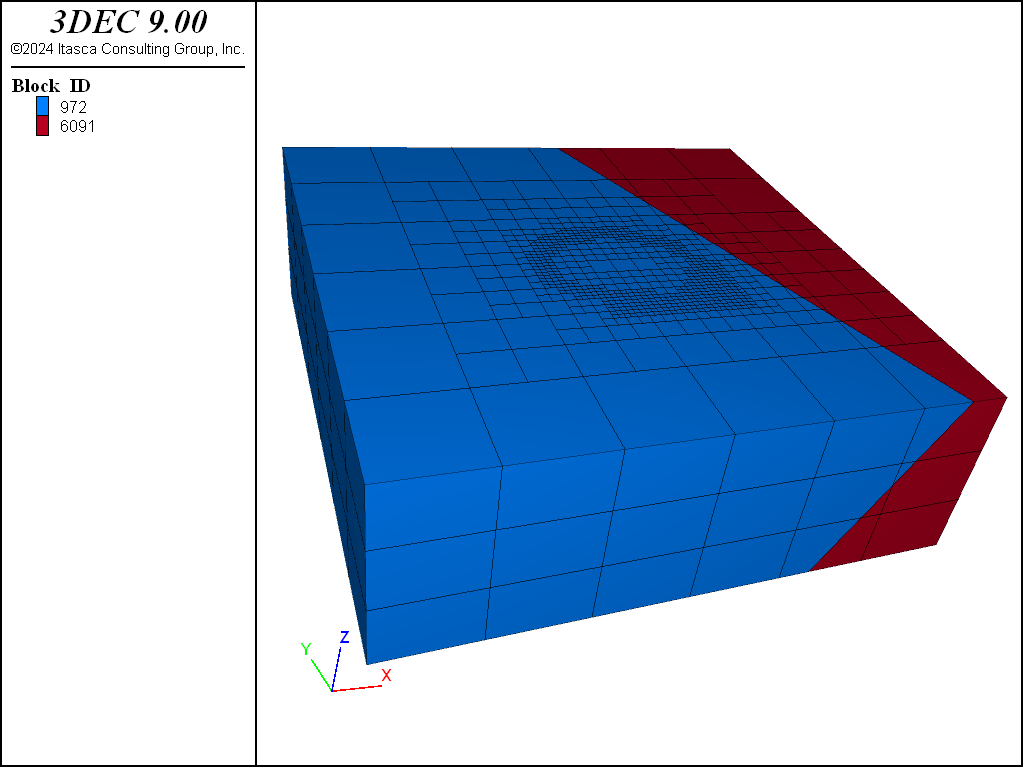
Figure 3: Blocks making up the open pit model after densification and cutting a fault.
Zoning and Properites
Now that the geometries and faults have been created, tetrahedral zoning can be performed. We want finer zoning around the pit and ore geometries and coarser zoning as we move concentrically away from the pit. We do this by first setting up groups to define the different regions and then using the block zone generate command specifying different edge sizes for the different groups.
We wish to assign different properties to the ore zone and the surrounding rock. We can group the zones that are inside of the ore geometry with the command block zone group 'ore_zones' range geometry-space 'ore' count odd.
The range geometry projects a ray from the centre of each zone and counts the number of intersections with the geometry. The default ray direction is vertical upward (0, 0, 1). Using the count odd keywords will cause zones to be added to the group if there are an odd number of intersections of the projected ray (i.e., zone inside the geometry).
The resulting zone groups are shown in Figure 4 shows ….
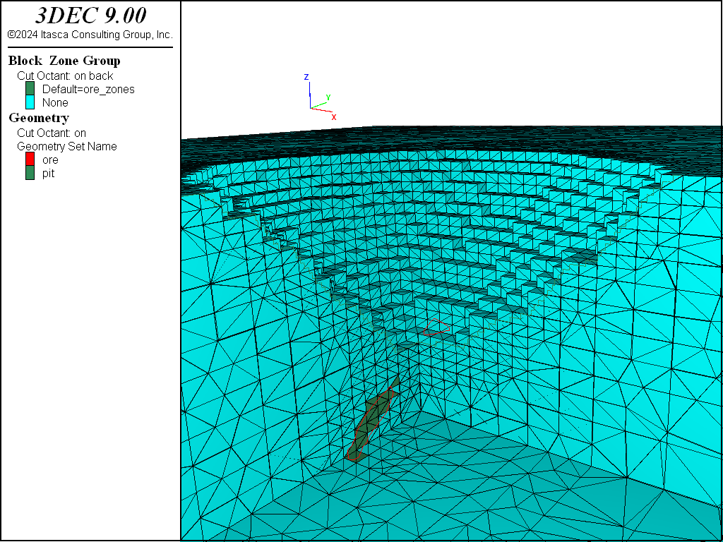
Figure 4: Zoned model showing zone groups. One quarter of the model is cut away for visualization.
Properties are then assigned to the zones as shown in the following table:
Property |
Host Rock |
Ore |
Units |
|---|---|---|---|
Constitutive Model |
Mohr-Coulomb |
Mohr-Coulomb |
|
Bulk Modulus |
2.5e8 |
5e7 |
lbf/ft^2 |
Shear Modulus |
1.5e8 |
2.3e7 |
lbf/ft^2 |
Density |
5.4 |
3.5 |
slugs/ft^3 |
Cohesion |
2.5e4 |
3e3 |
lbf/ft^2 |
Friction |
60 |
35 |
degrees |
Tension |
4e3 |
50 |
lbf/ft^2 |
Joint properties are also assigned to the fault. A friction of 20^{circ} and a cohesion of 1000 lbf/ft^2 is assigned.
Initial and Boundary Conditions
The model now requires gravity, in-situ stresses and boundary conditions to be initialized. This is done using the following commands:
model gravity 0 0 -32.17
;
block insitu topography ratio-x 1 ratio-y 1
;
block gridpoint apply velocity-x 0 range position-x 10000
block gridpoint apply velocity-x 0 range position-x 16000
block gridpoint apply velocity-y 0 range position-y -27000
block gridpoint apply velocity-y 0 range position-y -21000
block gridpoint apply velocity-z 0 range position-z -1620
The gravity parameter is set to 32.17 ft/sec2 in the downward z-direction (x and y components are 0). Insitu stresses are determined based on the rock density, depth and gravity using the block insitu topography command. The stresses are to be isotropic (ratio-x and ratio-y are set to 1.
Boundary conditions are established using the block gridpoint apply command. The extents of the model are restricted to zero velocity in the direction perpendicular to the boundary. The top of the model is free to move.
A final step is to turn on Nodal Mixed Discretization (block zone nodal-mixed-discretizaton on. This is a numerical technique used to obtain more accurate plasticity results from tetrahedral zones.
The model is then solved and saved.
Excavation
The next step is the grouping of the material inside the pit area. Initially, the block groups are reset and all blocks are assigned to a group called “default.”. We then assign the blocks inside the pit to a group called “pit” using a similar command to what was used with assigning the “ore” zone group. Note that we have to change the direction of the projecting ray to be downwards, so that the blocks above the pit are identified. The resulting block groups are shown in Figure 5 .
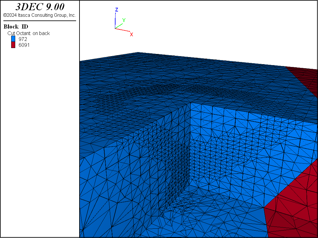
Figure 5: Zoned model showing block groups. One quarter of the model is cut away for visualization.
Now the pit material can be removed. Since the blocks within the pit geometry were grouped earlier, it is possible to easily excavate the range specified by the “pit_blocks” group (block excavate range group 'pit_blocks'.
Next, we reset the joint and gridpoint displacements since we don’t care about the displacement that occurred during initial stress installation. Finally the model is solved using model solve elastic. The elastic keyword will cause the model to be first solved with all joints and zones set to be elastic (no failure) and then solved again with true zone and joint strengths. This is useful to prevent spurious failure causes by unrealistic instantaneous stress changes when the entire pit is excavated at once.
Results
The resultng gridpoint displacements are shown in Figure 6. The displacement is generally upwards, reflecting the rebound due to removal of rock.
The joint displacement is shown in Figure 7. The joint displacements are small and deep, showin that there is no significant slip on the fault due to the pit excavation.
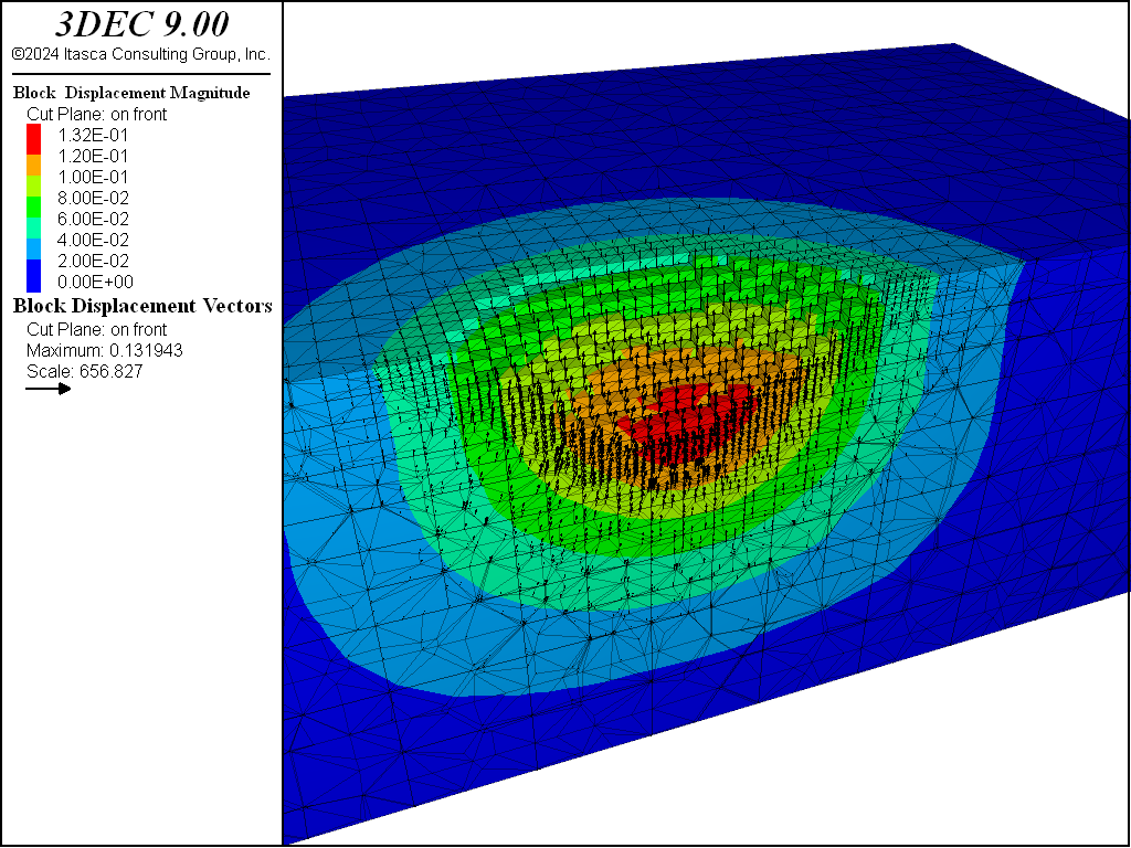
Figure 6: Displacements in the open pit model
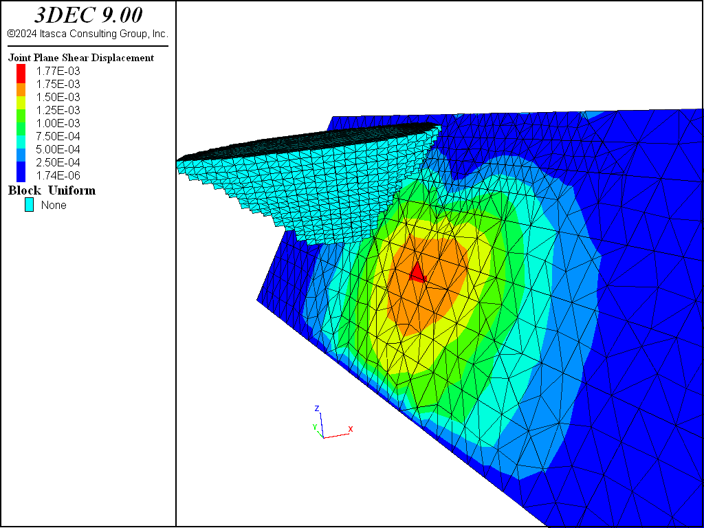
Figure 7: Shear displacements on a joint in the open pit model
Painting
After the model has been solved, you can perform post-analysis by plotting quantities at specific locations. 3DEC includes the ability to “paint” data on imported geometric surfaces. Suppose there was a critical tunnel under the pit and we wish to know the displacements on the tunnel. The tunnel itself is not actually modelled, but we can estimate the effect of the excavation at the tunnel location by painting displacements on to the tunnel surface.
We import a tunnel geometry “tunnel.stl”. Different properties can be “painted” onto existing geometry sets as if they were proposed and not yet constructed, or if these features exist but were not modelled. We will paint the displacement data onto the tunnel using the paint-extra-block keyword of the geometry command.
The results are shown in Figure 8.
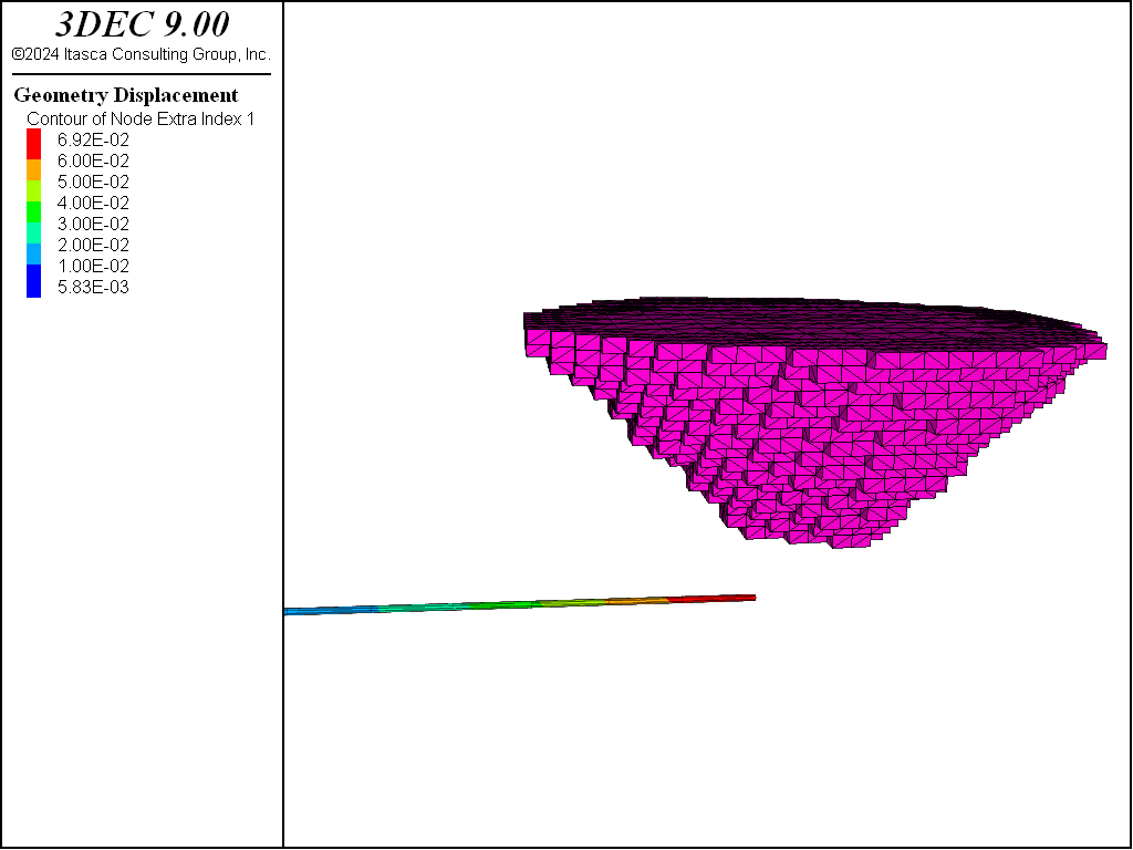
Figure 8: Displacements painted on to proposed tunnel
Data Files
octree_pit.dat
; ---- Example model of a pit excavation ----
model new
model random 10000
model large-strain on

block tolerance 0.01
block create brick (10000,16000 -27000,-21000 -1620,380)
;
block densify segments 6 6 3 join
;
; --- import geometries and densify blocks near the pit and ore boundaries --
geometry import 'pit.stl'
geometry import 'ore.stl'
;
block densify gradient-limit repeat 4 join ...
  range geometry-distance 'pit' set 'ore' gap 0 extent
;
; --- Add joint ---
block cut joint-set dip 60 dip-direction 250 origin 14200,-24300,-270
;
;
; --- Zone blocks ---
block group 'coarse_zone' range geometry-distance 'pit' set 'ore' gap 500
block group 'fine_zone' range geometry-distance 'pit' set 'ore' gap 100
block zone generate edgelength 50 range group 'fine_zone'
block zone generate edgelength 100 range group 'coarse_zone'
block zone generate edgelength 200
;
block zone group 'ore_zones' range geometry-space 'ore' count odd
;
; --- Set properties ---
block zone cmodel assign mohr-coulomb
block zone property bulk 2.5e8 shear 1.5e8 density 5.4
block zone property cohesion 25000 friction 60 tension 4000
block zone property bulk 5e7 shear 2.3e7 density 3.5 range group 'ore_zones'
block zone property cohesion 3000 friction 35 tension 50 ...
  range group 'ore_zones'
;
block contact property stiffness-normal 1e7 stiffness-shear 6e6 ...
  friction 20 cohesion 1000 tension 0
block contact material-table default property stiffness-normal 1e7 ...
  stiffness-shear 6e6
;
; --- Set up initial and boundary conditions ---
model gravity 0 0 -32.17
;
block insitu topography ratio-x 1 ratio-y 1
;
block gridpoint apply velocity-x 0 range position-x 10000
block gridpoint apply velocity-x 0 range position-x 16000
block gridpoint apply velocity-y 0 range position-y -27000
block gridpoint apply velocity-y 0 range position-y -21000
block gridpoint apply velocity-z 0 range position-z -1620
;
; --- Set NMD on ---
block zone nodal-mixed-discretization on
;
; --- solve initial state ---
model solve
model save 'pit_initial'

==================================================
;
block group 'default'
block group 'pit_blocks' range geometry-space 'pit' count 1 direction 0 0 -1
;
; --- Excavate and solve ---
block excavate range group 'pit_blocks'
block gridpoint initialize displacement 0 0 0
block contact reset displacement
model solve elastic

=================================================
;
; --- Paint displacements onto proposed tunnel ---
geometry import 'tunnel.stl'
geometry select 'tunnel'
geometry paint-extra-block 1 displacement component magnitude
;
model save 'pit_solve'
Endnotes
| Was this helpful? ... | Itasca Software © 2024, Itasca | Updated: Apr 02, 2024 |
