FLAC3D Theory and Background • Constitutive Models

Columnar-Basalt (COMBA) Model**

Note

**Not available in FLAC2D.

The Columnar-Basalt (COMBA) model (Detournay et al 2016, Meng et al 2020) accounts for the presence of up to four arbitrary orientations of weakness (ubiquitous joint) in a non-isotropic elastic matrix. The model can be applied to model quadrangular (hexagonal) columnar basalt with cross-joints by specifying that two (three) of the ubiquitous joints are oriented along the column axis, and another along the cross-joints. The model elastic behavior accounts for the compliance of the column matrix and that of the joints. The criterion for failure on the planes consists of a strain hardening/softening Coulomb envelope with tension cutoff; the strain hardening/softening behavior can be specified (using a table) for joint cohesion, friction, dilation, and tension. In addition, an amplification factor can be applied to joint dilation that depends on the angle between a set direction (i.e. the column mean axis) and the direction of slip on the joint. The amplification factor versus angle is specified in an input table.

Formulations

Definition of Joint Orientation, Spacing and Stiffness

The orientation of a joint is specified either by the dip (dip) and dip direction (dd) of the joint plane, or by the three components of the unit normal to the plane. Up to four joints planes can be considered.

The spacing of joint i is \(S_i\), the normal stiffness is \(k_i^n\), and the shear stiffness is \(k_i^s\) (the joint compliance terms related to normal and shear displacements under shear and normal loads are ignored).

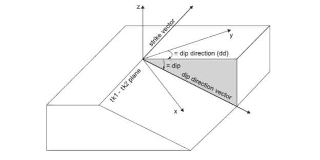
Figure 1: Definition of dip and dip direction for a joint plane in x-y-z reference axes.

Elastic Stress-Strain Behavior

The global elastic strain-stress relations used in the model logic are obtained by superposition of strain contributions from the column matrix and from the joints. The isotropic elastic column matrix has Young modulus, \(E\) and Poisson ratio, \(\nu\). The matrix contribution to the incremental strain-stress relations are expressed using Voigt notation as follows.

(1)\[\begin{split}\begin{Bmatrix} \dot{\epsilon}_{xx} \\ \dot{\epsilon}_{yy} \\ \dot{\epsilon}_{zz} \\ 2\dot{\epsilon}_{xy} \\ 2\dot{\epsilon}_{xz} \\ 2\dot{\epsilon}_{yz} \end{Bmatrix} = \begin{bmatrix} {{1}\over{E}} & -{{\nu}\over{E}} & -{{\nu}\over{E}} & & & \\ -{{\nu}\over{E}} & {{1}\over{E}} & -{{\nu}\over{E}} & & & \\ -{{\nu}\over{E}} & -{{\nu}\over{E}} & {{1}\over{E}} & & & \\ & & & {{1}\over{G}} & & \\ & & & & {{1}\over{G}} & \\ & & & & & {{1}\over{G}} \end{bmatrix} \begin{Bmatrix} \dot{\sigma}_{xx} \\ \dot{\sigma}_{yy} \\ \dot{\sigma}_{zz} \\ \dot{\sigma}_{xy} \\ \dot{\sigma}_{xz} \\ \dot{\sigma}_{yz} \end{Bmatrix}\end{split}\]

where \(G=E/2(1+\mu)\)

A local system of axes is defined for the joint; axis 3 is normal to the plane, 1 is in the direction of the dip direction vector, and 2, in the direction of the strike.

The stress and strain tensors transformation from local to global axes and vice-versa is obtained by application of the usual matrix transformation operations.

The local elastic strain increment contribution of the joint is expressed as follows.

(2)\[\begin{split}\begin{Bmatrix} \dot{\epsilon}^e_{xx} \\ \dot{\epsilon}^e_{yy} \\ \dot{\epsilon}^e_{zz} \\ 2\dot{\epsilon}^e_{xy} \\ 2\dot{\epsilon}^e_{xz} \\ 2\dot{\epsilon}^e_{yz} \end{Bmatrix} = \begin{bmatrix} 0 & 0 & 0 & 0 & 0 & 0 \\ 0 & 0 & 0 & 0 & 0 & 0 \\ 0 & 0 & 0 & 0 & 0 & 0 \\ 0 & 0 & 0 & {1}\over{k^s_iS_i} & 0 & 0 \\ 0 & 0 & 0 & 0 & {1}\over{k^s_iS_i} & 0 \\ 0 & 0 & 0 & 0 & 0 & {1}\over{k^s_iS_i} \end{bmatrix} \begin{Bmatrix} \dot{\sigma}_{xx} \\ \dot{\sigma}_{yy} \\ \dot{\sigma}_{zz} \\ \dot{\sigma}_{xy} \\ \dot{\sigma}_{xz} \\ \dot{\sigma}_{yz} \end{Bmatrix}\end{split}\]

The local compliance matrix, \(S^i_L\) (entity between brackets in Eq. (2)) is converted to global axes, and the result, \(S^i_L\) is added to the global compliance matrix. The transformation from local to global axes is performed using the matrix product:

(3)\[S^i_G = Q^i S^i_L Q^{iT}\]

where \(Q^i\) is the local-to-global strain transformation matrix for joint i, and \(Q^{iT}\) is the transpose of \(Q^i\). The final compliance matrix (i.e. the sum of matrix and joint contributions) is inverted to produce \(C_G\), the global elasticity matrix; the components of the global elasticity matrix are stored, taking into account the matrix symmetry. In addition, to save calculation time in small strain analyses, the elasticity matrix, \(C_G\) is expressed in the local axes of joint i, and the components of the resulting local matrix, \(C^i_L\) are stored, taking again into consideration the matrix symmetry. The transformation from global to local axes is performed using the matrix product:

(4)\[C^i_L = Q^{*i} C^i_G Q^{*iT}\]

where \(Q^{*i}\) is the global-to-local stress transformation matrix for joint i, and \(Q^{*iT}\) is the transpose of \(Q^{*i}\).

In the text below, we consider a particular joint, i and the incremental stress-strain relations in the local axes of that joint. The indices i, referring to the joint, and L, referring to the local axes are omitted to simplify the notation. With these conventions, the formal expression of the local stress strain relations in Voigt notation is:

(5)\[\begin{split}\begin{Bmatrix} \dot{\sigma}_{xx} \\ \dot{\sigma}_{yy} \\ \dot{\sigma}_{zz} \\ \dot{\sigma}_{xy} \\ \dot{\sigma}_{xz} \\ \dot{\sigma}_{yz} \end{Bmatrix} = \begin{bmatrix} C_{11} & C_{12} & C_{13} & C_{14} & C_{15} & C_{16} \\ C_{21} & C_{22} & C_{23} & C_{24} & C_{25} & C_{26} \\ C_{31} & C_{32} & C_{33} & C_{34} & C_{35} & C_{36} \\ C_{41} & C_{42} & C_{43} & C_{44} & C_{45} & C_{46} \\ C_{51} & C_{52} & C_{53} & C_{54} & C_{55} & C_{56} \\ C_{61} & C_{62} & C_{63} & C_{64} & C_{65} & C_{66} \end{bmatrix} \begin{Bmatrix} \dot{\epsilon}^e_{xx} \\ \dot{\epsilon}^e_{yy} \\ \dot{\epsilon}^e_{zz} \\ 2\dot{\epsilon}^e_{xy} \\ 2\dot{\epsilon}^e_{xz} \\ 2\dot{\epsilon}^e_{yz} \end{Bmatrix}\end{split}\]

The local strain (stress) components involved in the above relation are evaluated from the global strain (stress) tensors after application of the usual matrix transformation operations from global to local axes.

Yield Criterion and Flow Rule for a Weak Plane

The local yield criterion on a weak plane is the composite of a Coulomb criterion for slip, \(f^s\) and a tension cut-off, \(f^t\), i.e.,:

(6)\[f^s = \sqrt{\sigma_{13}^2 + \sigma_{23}^2} + \sigma_{33}\tan{\phi} - c\]

and

(7)\[f^t = \sigma_{33} - \sigma^t\]

where \(\phi\) is joint friction, c is joint cohesion, and \(\sigma^t\) is joint tensile strength. For a joint with non-zero friction angle, the tensile strength is capped with the maximum value of \(c/\tan(\phi)\).

Shear yielding on a weak plane corresponds to a non-associated flow rule; the potential function is:

(8)\[g^s = \sqrt{\sigma_{13}^2 + \sigma_{23}^2} + \sigma_{33}\tan{\psi}\]

where \(\psi\) is the joint dilation.

Tension yielding on a weak plane corresponds to an associated flow rule, and the potential function is:

(9)\[g^t = \sigma_{33}\]

For simplicity of notation in the text below, we use the following notation:

(10)\[\tau_3 = \sqrt{\sigma_{13}^2 + \sigma_{23}^2}\]

The flow rule is obtained, as usual, by differentiation of the potential function with respect to the stress components. The incremental plastic stain components for shear yielding on a weak plane thus are obtained from Eq. (8):

(11)\[\begin{split}\begin{array}{l} \dot{\sigma}_{11}^p = \dot{\sigma}_{22}^p = \dot{\sigma}_{12}^p = 0 \\ \dot{\sigma}_{33}^p = \lambda^s \tan{\psi} \\ \dot{\sigma}_{12}^p = \lambda^s {\sigma_{12}}/{\tau_3} \\ \dot{\sigma}_{13}^p = \lambda^s {\sigma_{13}}/{\tau_3} \end{array}\end{split}\]

For tension yielding on weak planes, the incremental plastic strain components are derived from (9):

(12)\[\begin{split}\begin{array}{l} \dot{\sigma}_{11}^p = \dot{\sigma}_{22}^p = \dot{\sigma}_{12}^p = \dot{\sigma}_{13}^p = \dot{\sigma}_{23}^p = 0 \\ \dot{\sigma}_{33}^p = \lambda^t \end{array}\end{split}\]

We recall that the FLAC3D/3DEC calculation scheme proceeds in incremental computational steps. At each step, the constitutive model receives the old stress (obtained at the end of the previous step) as input and the total strain increment for the step, and it is in charge of producing the new stress value for the current step. In the model implementation, an elastic guess for the stress is computed first using the total strain increment. The yield conditions are tested on the weak planes. If yielding is detected, a stress correction is applied to the elastic guess that is consistent with plasticity theory, as follows.

As usual, the total strain increment is expressed as the sum of elastic and plastic components. According to this superposition principle, the local stress-strain Eq. (5) can be expressed as follows.

(13)\[\begin{split}\begin{Bmatrix} \dot{\sigma}_{xx} \\ \dot{\sigma}_{yy} \\ \dot{\sigma}_{zz} \\ \dot{\sigma}_{xy} \\ \dot{\sigma}_{xz} \\ \dot{\sigma}_{yz} \end{Bmatrix} = \begin{bmatrix} C_{11} & C_{12} & C_{13} & C_{14} & C_{15} & C_{16} \\ C_{21} & C_{22} & C_{23} & C_{24} & C_{25} & C_{26} \\ C_{31} & C_{32} & C_{33} & C_{34} & C_{35} & C_{36} \\ C_{41} & C_{42} & C_{43} & C_{44} & C_{45} & C_{46} \\ C_{51} & C_{52} & C_{53} & C_{54} & C_{55} & C_{56} \\ C_{61} & C_{62} & C_{63} & C_{64} & C_{65} & C_{66} \end{bmatrix} \begin{Bmatrix} \dot{\epsilon}_{xx} \\ \dot{\epsilon}_{yy} \\ \dot{\epsilon}_{zz} \\ 2\dot{\epsilon}_{xy} \\ 2\dot{\epsilon}_{xz} \\ 2\dot{\epsilon}_{yz} \end{Bmatrix} \\ - \begin{bmatrix} C_{11} & C_{12} & C_{13} & C_{14} & C_{15} & C_{16} \\ C_{21} & C_{22} & C_{23} & C_{24} & C_{25} & C_{26} \\ C_{31} & C_{32} & C_{33} & C_{34} & C_{35} & C_{36} \\ C_{41} & C_{42} & C_{43} & C_{44} & C_{45} & C_{46} \\ C_{51} & C_{52} & C_{53} & C_{54} & C_{55} & C_{56} \\ C_{61} & C_{62} & C_{63} & C_{64} & C_{65} & C_{66} \end{bmatrix} \begin{Bmatrix} \dot{\epsilon}^p_{xx} \\ \dot{\epsilon}^p_{yy} \\ \dot{\epsilon}^p_{zz} \\ 2\dot{\epsilon}^p_{xy} \\ 2\dot{\epsilon}^p_{xz} \\ 2\dot{\epsilon}^p_{yz} \end{Bmatrix}\end{split}\]

The stress increments in Eq. (13) stand for the difference between new (N) and old (O) stress for the step:

(14)\[\begin{split}\begin{Bmatrix} \Delta{\sigma}_{xx} \\ \Delta{\sigma}_{yy} \\ \Delta{\sigma}_{zz} \\ \Delta{\sigma}_{xy} \\ \Delta{\sigma}_{xz} \\ \Delta{\sigma}_{yz} \end{Bmatrix} = \begin{Bmatrix} {\sigma}_{xx}^N \\ {\sigma}_{yy}^N \\ {\sigma}_{zz}^N \\ {\sigma}_{xy}^N \\ {\sigma}_{xz}^N \\ {\sigma}_{yz}^N \end{Bmatrix} - \begin{Bmatrix} {\sigma}_{xx}^O \\ {\sigma}_{yy}^O \\ {\sigma}_{zz}^O \\ {\sigma}_{xy}^O \\ {\sigma}_{xz}^O \\ {\sigma}_{yz}^O \end{Bmatrix}\end{split}\]

After substitution of Eq. (14) in Eq. (13), and some manipulation, we write:

(15)\[\begin{split}\begin{Bmatrix} {\sigma}_{xx}^N \\ {\sigma}_{yy}^N \\ {\sigma}_{zz}^N \\ {\sigma}_{xy}^N \\ {\sigma}_{xz}^N \\ {\sigma}_{yz}^N \end{Bmatrix} = \begin{Bmatrix} {\sigma}_{xx}^G \\ {\sigma}_{yy}^G \\ {\sigma}_{zz}^G \\ {\sigma}_{xy}^G \\ {\sigma}_{xz}^G \\ {\sigma}_{yz}^G \end{Bmatrix} - \begin{Bmatrix} {\sigma}_{xx}^C \\ {\sigma}_{yy}^C \\ {\sigma}_{zz}^C \\ {\sigma}_{xy}^C \\ {\sigma}_{xz}^C \\ {\sigma}_{yz}^C \end{Bmatrix}\end{split}\]

where the (known) elastic guess (G) for the step is:

(16)\[\begin{split}\begin{Bmatrix} {\sigma}_{xx}^G \\ {\sigma}_{yy}^G \\ {\sigma}_{zz}^G \\ {\sigma}_{xy}^G \\ {\sigma}_{xz}^G \\ {\sigma}_{yz}^G \end{Bmatrix} = \begin{Bmatrix} {\sigma}_{xx}^O \\ {\sigma}_{yy}^O \\ {\sigma}_{zz}^O \\ {\sigma}_{xy}^O \\ {\sigma}_{xz}^O \\ {\sigma}_{yz}^O \end{Bmatrix} + \begin{bmatrix} C_{11} & C_{12} & C_{13} & C_{14} & C_{15} & C_{16} \\ C_{21} & C_{22} & C_{23} & C_{24} & C_{25} & C_{26} \\ C_{31} & C_{32} & C_{33} & C_{34} & C_{35} & C_{36} \\ C_{41} & C_{42} & C_{43} & C_{44} & C_{45} & C_{46} \\ C_{51} & C_{52} & C_{53} & C_{54} & C_{55} & C_{56} \\ C_{61} & C_{62} & C_{63} & C_{64} & C_{65} & C_{66} \end{bmatrix} \begin{Bmatrix} \Delta{\epsilon}_{xx} \\ \Delta{\epsilon}_{yy} \\ \Delta{\epsilon}_{zz} \\ 2\Delta{\epsilon}_{xy} \\ 2\Delta{\epsilon}_{xz} \\ 2\Delta{\epsilon}_{yz} \end{Bmatrix}\end{split}\]

And the stress correction (C), yet to be determined is:

(17)\[\begin{split}\begin{Bmatrix} {\sigma}_{xx}^C \\ {\sigma}_{yy}^C \\ {\sigma}_{zz}^C \\ {\sigma}_{xy}^C \\ {\sigma}_{xz}^C \\ {\sigma}_{yz}^C \end{Bmatrix} = \begin{bmatrix} C_{11} & C_{12} & C_{13} & C_{14} & C_{15} & C_{16} \\ C_{21} & C_{22} & C_{23} & C_{24} & C_{25} & C_{26} \\ C_{31} & C_{32} & C_{33} & C_{34} & C_{35} & C_{36} \\ C_{41} & C_{42} & C_{43} & C_{44} & C_{45} & C_{46} \\ C_{51} & C_{52} & C_{53} & C_{54} & C_{55} & C_{56} \\ C_{61} & C_{62} & C_{63} & C_{64} & C_{65} & C_{66} \end{bmatrix} \begin{Bmatrix} \Delta{\epsilon}_{xx}^p \\ \Delta{\epsilon}_{yy}^p \\ \Delta{\epsilon}_{zz}^p \\ 2\Delta{\epsilon}_{xy}^p \\ 2\Delta{\epsilon}_{xz}^p \\ 2\Delta{\epsilon}_{yz}^p \end{Bmatrix}\end{split}\]

Clearly, various yielding scenarios are possible in each computational step. In fact, hundreds of different cases can be recorded, including single and simultaneous shear yielding on 1, 2, 3 or 4 weak planes, single and simultaneous tensile yielding on one or more weak planes, and combined shear and tensile yielding on one or more weak planes. To simplify the coding, it seems reasonable to focus attention at each computational step, on the weak plane exhibiting the most severe case of shear yielding, and that (same or different) with the largest potential amount of tensile yielding, and make the appropriate stress correction. Presumably, the yielding not ‘caught’ in one step will be addressed in the steps that follow.

With this idea in mind, we are down to consider two yielding scenarios to evaluate local stress corrections: 1) shear yielding only on a single weak plane (3 cases) and 2) tensile yielding only on a single yield plane (3 cases).

Shear Yielding on a Weak Plane

The case of shear yielding only on a weak plane is considered in this section. After substitution in Eq. (17)) of the plastic strain increments in Eq. (11), we obtain the following stress corrections for shear yielding on a joint.

(18)\[\begin{split}\begin{array}{l} {\sigma}_{11}^C = \lambda^s ( C_{13}\tan{\psi} + 2C_{15} \frac{\sigma_{13}}{\tau_3} + 2C_{16} \frac{\sigma_{23}}{\tau_3} ) \\ {\sigma}_{22}^C = \lambda^s ( C_{23}\tan{\psi} + 2C_{25} \frac{\sigma_{13}}{\tau_3} + 2C_{26} \frac{\sigma_{23}}{\tau_3} ) \\ {\sigma}_{33}^C = \lambda^s ( C_{33}\tan{\psi} + 2C_{35} \frac{\sigma_{13}}{\tau_3} + 2C_{36} \frac{\sigma_{23}}{\tau_3} ) \\ {\sigma}_{12}^C = \lambda^s ( C_{34}\tan{\psi} + 2C_{45} \frac{\sigma_{13}}{\tau_3} + 2C_{46} \frac{\sigma_{23}}{\tau_3} ) \\ {\sigma}_{13}^C = \lambda^s ( C_{35}\tan{\psi} + 2C_{55} \frac{\sigma_{13}}{\tau_3} + 2C_{56} \frac{\sigma_{23}}{\tau_3} ) \\ {\sigma}_{23}^C = \lambda^s ( C_{36}\tan{\psi} + 2C_{56} \frac{\sigma_{13}}{\tau_3} + 2C_{66} \frac{\sigma_{23}}{\tau_3} ) \end{array}\end{split}\]

The magnitude of \(\lambda^s\) is determined from the condition that the new (corrected) stresses (N) must satisfy the condition for shear yielding, see Eq. (7). The new stresses for the step, obtained from Eq. (15) and Eq. (18), are as follows.

(19)\[\begin{split}\begin{array}{l} {\sigma}_{11}^N = {\sigma}_{11}^G - \lambda^s ( C_{13}\tan{\psi} + 2C_{15} \frac{\sigma_{13}}{\tau_3} + 2C_{16} \frac{\sigma_{23}}{\tau_3} ) \\ {\sigma}_{22}^N = {\sigma}_{22}^G - \lambda^s ( C_{23}\tan{\psi} + 2C_{25} \frac{\sigma_{13}}{\tau_3} + 2C_{26} \frac{\sigma_{23}}{\tau_3} ) \\ {\sigma}_{33}^N = {\sigma}_{33}^G - \lambda^s ( C_{33}\tan{\psi} + 2C_{35} \frac{\sigma_{13}}{\tau_3} + 2C_{36} \frac{\sigma_{23}}{\tau_3} ) \\ {\sigma}_{12}^N = {\sigma}_{12}^G - \lambda^s ( C_{34}\tan{\psi} + 2C_{45} \frac{\sigma_{13}}{\tau_3} + 2C_{46} \frac{\sigma_{23}}{\tau_3} ) \\ {\sigma}_{13}^N = {\sigma}_{13}^G - \lambda^s ( C_{35}\tan{\psi} + 2C_{55} \frac{\sigma_{13}}{\tau_3} + 2C_{56} \frac{\sigma_{23}}{\tau_3} ) \\ {\sigma}_{23}^N = {\sigma}_{23}^G - \lambda^s ( C_{36}\tan{\psi} + 2C_{56} \frac{\sigma_{13}}{\tau_3} + 2C_{66} \frac{\sigma_{23}}{\tau_3} ) \end{array}\end{split}\]

After substitution of \({\sigma}_{ij}^N\) in Eq. (19) for \({\sigma}_{ij}\) in Eq. (6), the criteria for shear yielding can be expressed as:

(20)\[\sqrt{(a_1 - a_2 \lambda^s)^2 + (a_3 - a_4 \lambda^s)^2} - a_5 \lambda^s + a_6 = 0\]

with the constants \(a_i\) (i=1,6) defined as follows:

(21)\[\begin{split}\begin{array}{l} a_1 = {\sigma}_{13}^G \\ a_2 = C_{33}\tan{\psi} + 2C_{35} \frac{\sigma_{13}}{\tau_3} + 2C_{36} \frac{\sigma_{23}}{\tau_3} \\ a_3 = {\sigma}_{23}^G \\ a_4 = C_{34}\tan{\psi} + 2C_{45} \frac{\sigma_{13}}{\tau_3} + 2C_{46} \frac{\sigma_{23}}{\tau_3} \\ a_5 = ( C_{33}\tan{\psi} + 2C_{35} \frac{\sigma_{13}}{\tau_3} + 2C_{36} \frac{\sigma_{23}}{\tau_3} ) \tan{\phi} \\ a_6 = {\sigma}_{33}^G \tan{\phi} - c \end{array}\end{split}\]

Solving Eq. (20) for the smallest root, we obtain:

(22)\[\begin{split}\begin{array}{l} A \neq 0: \; \lambda^s = \frac{B}{A} - \sqrt{(\frac{B}{A})^2 - \frac{C}{A}} \\ A = 0: \; \lambda^s = \frac{C}{2B} \end{array}\end{split}\]

with

(23)\[\begin{split}\begin{array}{l} A = a_2^2 + a_4^2 - a_5^2 \\ B = a_1a_2 + a_3d_4 - a_5a_6 \\ C = a_1^2 + a_3^2 - a_6^2 \end{array}\end{split}\]

After \(\lambda^s\) has been calculated using (22), the plastic corrections for the local stress components on the weak plane are defined from (19).

Note that in the current implementation of the model the coefficient \(a_2\) , \(a_4\) and \(a_5\) are computed using the elastic guess for the step. The accuracy of \(\lambda^s\) could potentially be improved by performing iterations between Eqs. (21) and (22) after updating the value of \(a_2\) , \(a_4\) and \(a_5\) using new computed stress values until convergence is achieved. However, this does not seem necessary (see verification tests below) as the computational steps are typically small enough.

Tensile Yielding on a Weak Plane

For tensile failure only on a single weak plane, we follow the same procedure. After substitution in Eq. (17) of the plastic strain increment for tensile yielding listed in (7), the stress corrections change are as follows:

(24)\[\begin{split}\begin{array}{l} \sigma_{11}^C = \lambda^t C_{13} \\ \sigma_{22}^C = \lambda^t C_{23} \\ \sigma_{33}^C = \lambda^t C_{33} \\ \sigma_{12}^C = \lambda^t C_{34} \\ \sigma_{13}^C = \lambda^t C_{35} \\ \sigma_{23}^C = \lambda^t C_{36} \end{array}\end{split}\]

The magnitude of \(\lambda^t\) is determined from the condition that the new (corrected) stresses (N) must satisfy the condition for tensile yielding, see Eq. (7). The new normal stress on the joint for the step is obtained from Eq. (13) and Eq. (24):

(25)\[\begin{split}\begin{array}{l} \sigma_{11}^N = \sigma_{11}^G - \lambda^t C_{13} \\ \sigma_{22}^N = \sigma_{22}^G - \lambda^t C_{23} \\ \sigma_{33}^N = \sigma_{33}^G - \lambda^t C_{33} \\ \sigma_{12}^N = \sigma_{12}^G - \lambda^t C_{34} \\ \sigma_{13}^N = \sigma_{13}^G - \lambda^t C_{35} \\ \sigma_{23}^N = \sigma_{23}^G - \lambda^t C_{36} \end{array}\end{split}\]

After application of the tensile yield criterion, using the expressions for normal stress on the joint listed in (25), and solving for \(\lambda^t\), we have:

(26)\[\lambda^t = \frac{\sigma_{33}^G - \sigma^t}{C_{33}}\]

The stress corrections for tensile yielding on individual plane listed in Eq. (24) now can be expressed in terms of known quantities.

Strain hardening/softening

The joint cohesion, friction, dilation and tensile strength may harden or soften after the onset of plastic yield. The user defines the joint cohesion, friction, and dilation as piecewise-linear function of an evolution parameter measuring the plastic shear strain. A piecewise-linear softening law for the tensile strength can also be prescribed in terms of another hardening parameter measuring the plastic tensile strength. The code measures the total plastic shear and tensile strains by incrementing the evolution parameters at each time step, and causes the model properties to conform to the user defined functions.

The parameter increment for measuring the plastic shear strain is the square root of the second invariant ( \(\sqrt{J^{\prime}_2}\)) of the incremental plastic shear-strain deviatoric tensor for the step:

(27)\[\Delta \kappa^s_j = \sqrt{\frac{1}{3}(\Delta{\epsilon}^p_{33})^2 + (\Delta{\epsilon}^p_{13})^2 + (\Delta{\epsilon}^p_{23})^2}\]

where the plastic strain components are given by (11).

The parameter increment for measuring the plastic tensile strain is the plastic volumetric tensile strain increment:

(28)\[\Delta \kappa^t_j = \Delta{\epsilon}^p_{33}\]

where the plastic strain increment is given by (12).

Directional dilation

Dilation is expected to be quite different if the direction of shear on a ‘lateral’ joint (i.e. a joint parallel to the column axis) is along the column axis, or normal to it. To represent this behavior, the user provides the three components of the unit vector along the mean column axis, and a table giving (a piece-wise linear representation of) the dilation amplification factor versus amplification angle (in degree) between the specified unit vector and the direction of slip on a joint. The dilation for the step is evaluated from the dilation table, if it is provided, and the value is multiplied by the amplification factor (the code calculates the amplification angle from the dot product of the unit vector and the slip direction vector, and the factor is found by interpolation, using the table provided.)

Large-Strain Update of Weak Plane Orientation

In large strain, the orientation of the weak planes possibly could be adjusted in each zone to account for rigid body rotations, and rotations due to deformations. However, this correction has not been considered in the current model implementation; it is left for future development.

Implementation Procedure

The implementation of the model proceeds as follows. The coefficients of the global elasticity matrix are computed and stored in the initialization phase. The local elasticity matrix of active joints are also stored. New stresses are estimated using the global elasticity matrix and the total strain increments for the step. The global stress tensor then is resolved in the local axes of the weak plane, and the local yield conditions are tested. If yielding is detected, a relevant local stress correction (derived using the flow rule) is calculated as described above. The stress correction then is resolved into global axes and subtracted from the global elastic stress estimate. The evolution parameters are incremented, and the strength properties are updated using the information in the input tables, as appropriate. Also, the dilation amplification factor is accounted for, as described above, if an amplification table is provided.

Creep Option

A creep rate component is added to the COMBA ubiquitous joints logic. We consider the power law suggested by Malan et al. (1998) that provides the following relation between steady state creep rate and the stress/strength ratio:

(29)\[\dot{\epsilon}^{cr} = A \left( \frac{\bar{\tau}}{\bar{\tau}_{max}} \right)^n\]

where \(\tau\) and \(\tau_{max}\) are the shear stress and maximum shear stress on the joint, respectively, the overbar stands for absolute value, and A and n are calibration parameters that depends on the absolute stress level (as well as the thickness and type of filling).

A local system of axes is defined for the joint; axis 3 is normal to the plane, axis 1 is in the direction of the dip direction vector, and axis 2 is in the direction of the strike. With this convention, the local shear stress on the joint is evaluated as follows:

(30)\[\bar{\tau} = \sqrt{\sigma^2_{13} + \sigma^2_{23}}\]

and the shear strength is calculated using Mohr criterion,

(31)\[\tau_{max} = c_j - \sigma_{33} \tan{\phi_j}\]

where compressive stresses are negative, \(c_j\) is joint friction, and \(\phi_j\) is joint friction.

In the COMBA implementation, creep only takes place if the normal stress on the joint, \(\sigma_{33}\), is compressive (\(\sigma_{33}\) is negative in this case). Also, the law uses a threshold ratio, \(s_{lim}\), above which creep is active (and below which creep does not take place):

(32)\[\frac{\bar{\tau}}{\bar{\tau}_{max}} > s_{lim}\]

where, e.g., \(s_{lim}=30\%\) for unfilled joints, and \(s_{lim}=10\%\) for filled joints (Glamheden, R., and H. Hokmark, 2010).

Finally, the local creep rate components in the joint plane are expressed as follows.

(33)\[\dot{\epsilon}^{cr}_{13} = \frac{\sigma_{13}}{\bar{\tau}} \dot{\epsilon}^{cr}, \;\;\; \dot{\epsilon}^{cr}_{23} = \frac{\sigma_{23}}{\bar{\tau}} \dot{\epsilon}^{cr}\]

The total strain increment is expressed as the sum of elastic, creep, and plastic components. Consistent with the superposition principle, the global (using a subscript G) stress-strain equations are expressed as follows:

(34)\[\{\Delta \sigma\}_G = C_G \{\Delta \epsilon\}_G - C_G \{\Delta \epsilon^{cr}\}_G \Delta t - C_G \{\Delta \epsilon^p\}_G\]

where the creep component is evaluated as the sum of joint contributions, and \(\Delta t\) is the creep timestep. By convention, we refer to the first, second, and third term in the right hand side of (34) as elastic guess, creep stress correction, and plastic stress correction, respectively:

(35)\[\begin{split}\{\Delta \sigma\}_G^{guess} = C_G \{\Delta \epsilon\}_G \\ \{\Delta \sigma^{cr}\}_G = C_G \{\dot{\epsilon}^{cr}\}_G \Delta t \\ \{\Delta \sigma^p\}_G = C_G \{\Delta \epsilon^p\}_G\end{split}\]

In the COMBA formulation, the creep contribution to the creep stress correction from joint i is evaluated in the local axes of the joint:

(36)\[\{\Delta \sigma^{i,cr}\}_L = C_L \{\dot{\epsilon}^{i,cr}\}_L \Delta t\]

where

(37)\[\{\dot{\epsilon}^{i,cr}\}_L = \{ 0, 0, 0, 0, 2\sigma^{i,cr}_{13}, 2\sigma^{i,cr}_{23}\}^i_L\]

The local contribution of joint i to the creep stress correction is then evaluated in global axes and added to the global contributions of the other joints in the model to provide the total creep stress correction for the step. The creep stress correction is subtracted from the elastic guess before the plastic stress correction is performed.

References

Detournay, C., Meng, G.T., & Cundall, P.A. “Development of a Constitutive Model for Columnar Basalt.” In: Proceedings of the 4th Itasca Symposium on Applied Numerical Modeling. (2016).

Glamheden, R. & Hokmark, H. Creep in jointed rock masses – State of knowledge. Svenk Karnbranslehantering AB, Swedish Nuclear Fuel and Waste Management Co. ISSN 1402-3091, SKB R-06-94. (2010).

Malan, D.F., Drescher, K., &Vogler, U.W. “Shear creep of discontinuities in hard rock surrounding deep excavations.” In: Rossmanith H-P (ed). Proceedings of the Third International Conference on Mechanics of Jointed and Faulted Rock – MJFR-3, Vienna, Austria, 6-9 April 1998. Rotterdam: Balkema, pp473-478. (1998).

Meng G.T., Detournay C. and Cundall P. “Formulation and Application of a Constitutive Model for Multijointed Material to Rock Mass Engineering.” International Journal of Geomechanics, 20(6) (2020).

columnar-basalt Model Properties

Use the following keywords with the zone property (FLAC3D) or block zone property (3DEC) command to set these properties of the Columnar-Basalt model.

columnar-basalt

cohesion f

matrix cohesion, \(c\) = \(c_1\).

dilation f

matrix dilation angle, \(\psi\) = \(\psi_1\). The default is 0.0.

dip-i f

dip angle [degrees] of weakness plane of the i-th (i=1,2,3,or 4) set.

dip-direction-i f

dip direction [degrees] of weakness plane of the i-th (i=1,2,3,or 4) set.

friction f

matrix friction angle, \(\phi\) = \(\phi_1\).

joint-cohesion-i f

joint cohesion, \(c_j\) of the i-th (i=1,2,3,or 4) set.

joint-dilation-i f

joint dilation angle, \(\psi_j\) of the i-th (i=1,2,3,or 4) set. The default is 0.0.

joint-friction-i f

joint friction angle of the i-th (i=1,2,3,or 4) set, \(\phi_j\).

joint-tension-i f

joint tension limit, \(\sigma^t_j\) of the i-th (i=1,2,3,or 4) set. The default is 0.0.

normal-x-amplification f

\(x\)-component of reference unit vector for amplification.

normal-y-amplification f

\(y\)-component of reference unit vector for amplification.

normal-z-amplification f

\(z\)-component of reference unit vector for amplification.

normal-x-i f

\(x\)-component of the normal direction to the weakness plane, \(n_x\), of the i-th (i=1,2,3,or 4) set.

normal-y-i f

\(y\)-component of the normal direction to the weakness plane, \(n_y\) of the i-th (i=1,2,3,or 4) set.

normal-z-i f

\(z\)-component of the normal direction to the weakness plane, \(n_z\) of the i-th (i=1,2,3,or 4) set.

poisson f

Poisson ratio for the column matrix.

space-i f

Space for joint of the i-th (i=1,2,3,or 4) set, \(S_i\). \(S_i\) = 0 (default value) means joint i (1,2,3, or 4) is inactive. \(S_i\) > 0 means the joint is active for detection of shear and tensile yielding. However, it may not contribute to the stiffness matrix, if \(k_{n,i} = k_{n,i} = 0\).

stiffness-normal-i f

Normal stiffness of joint of the i-th (i=1,2,3,or 4) set, \(k_{n,i}\).

stiffness-shear-i f

Shear stiffness of joint of the i-th (i=1,2,3,or 4) set, \(k_{s,i}\).

table-amplification f

Amplification table for joint dilation 1, 2, 3. It should provide entries between 0 and 90 degree. Dilation amplification factor affects joint 1 to 3. Presumably, the cross joint is not affected by dilation amplification, thus if present, it should be declared as joint 4.

tension f

tension limit, \({\sigma}^t\). The default is 0.0.

young f

Young’s modulus for the column matrix.

flag-matrix-plastic b (a)

If true, the matrix plasticity will be considered, otherwise the matrix is elastic. The default is false.

creep-coefficient-i f (a)

Creep parameter \(A\) of joint of the i-th (i=1,2,3,or 4) set. Valid only when creep is configured.

creep-exponent-i f (a)

Creep parameter \(n\) of joint of the i-th (i=1,2,3,or 4) set. Valid only when creep is configured.

creep-limit-ratio-i f (a)

Creep parameter \(s_{lim}\) of joint of the i-th (i=1,2,3,or 4) set. Valid only when creep is configured.

table-cohesion-i s (a)

name of the table relating matrix cohesion \(c\) = \(c_1\) to matrix plastic shear strain.

table-dilation-i s (a)

name of the table relating matrix dilation angle \(\psi\) = \(\psi_{1}\) to matrix plastic shear strain.

table-friction-i s (a)

name of the table relating matrix friction \(\psi\) = \(\psi_{1}\) angle to matrix plastic shear strain.

table-joint-cohesion-i s (a)

name of the table relating joint cohesion \(c_j\) = \(c_{j1}\) to joint plastic shear strain of the i-th (i=1,2,3,or 4) set.

table-joint-dilation-i s (a)

name of the table relating joint dilation \(\psi_j\) = \(\psi_{j1}\) to joint plastic shear strain of the i-th (i=1,2,3,or 4) set.

table-joint-friction-i s (a)

name of the table relating joint friction angle \(\phi_j\) = \(\phi_{j1}\) to joint plastic shear strain of the i-th (i=1,2,3,or 4) set.

table-joint-tension s (a)

name of the table relating joint tension limit \(\sigma^t_j\) to joint plastic tensile strain of the i-th (i=1,2,3,or 4) set.

strain-shear-plastic-joint-i f (r)

accumulated joint plastic shear strain of the i-th (i=1,2,3,or 4) set.

strain-tensile-plastic-joint-i f (r)

accumulated joint plastic tensile strain of the i-th (i=1,2,3,or 4) set.

Notes

• Any two active joints should not be parallel (i.e. have the same dip and dip direction, or the same unit normal),there is no automatic detection for this condition in the current version of the model, the user should make sure it is avoided.

• The Joint numbering is arbitrary (also, some of the joints may be not be present). However, the particularity of joint 4 is that it is not affected by dilation amplification.

• The tension cut-off is \({\sigma}^t = min({\sigma}^t, c/\tan \phi)\).

• The joint tension limit used in the model is the minimum of the input \(\sigma^t\) and \({c_j}/{\tan \phi_j}\) of the i-th (i=1,2,3,or 4) set.