FLAC3D Theory and Background • Constitutive Models

Von-Mises Model

The yield envelope for this model involves a von-Mises criterion. The position of a stress point on this envelope is controlled by an associated flow rule for shear failure.

Formulations

The yield function of the von-Mises model with kinematic hardening is defined as

(1)\[ f^s = \left[ 1.5 (s_{ij}-\alpha_{ij}) (s_{ij}-\alpha_{ij}) \right]^{0.5} - \sigma_Y = 0\]

where the Einstein summation convention applies, \(s_{ij}\) is the deviatoric stress tensor, \(\alpha_{ij}\) is the back-stress tensor under the condition \(\alpha_{ii}=0\)), and \(\sigma_Y\) is a positive material constant denoting yield strength under uniaxial conditions. Note that if there is no hardening, or \(\alpha_{ij} = 0\), the yield function becomes

(2)\[ f^s = q - \sigma_Y = 0\]

where \(q = ( 1.5\ s_{ij} s_{ij} )^{0.5}\).

Incremental Elastic Law

The incremental expression of Hooke’s law, in terms of the generalized stress and stress increments, has the form

(3)\[ \Delta s_{ij} = 2G \Delta e^e_{ij}\]

and

(4)\[ \Delta p = -3K \Delta \varepsilon^e_v\]

where \(p=-\sigma_{ii}/3\), \(G\) is the elastic shear modulus, \(K\) is the elastic bulk modulus, \(e^e_{ij}\) is the elastic part of deviatoric strain tensor, and \(\varepsilon^e_v\) is the elastic part of volumetric strain.

Composite Failure Criterion and Flow Rule

The potential function \(g^s\) corresponds in general to an associated law, and has the form

(5)\[ g^s = f^s\]

Hardening Rule

The hardening rule is assumed

(6)\[ \Delta \alpha_{ij} = H \Delta \epsilon^p_{ij}\]

where \(H\) is a material constant called kinematic plastics modulus. See the schematic in Figure 1 for the physical meaning of the plastic modulus in uniaxial loading.

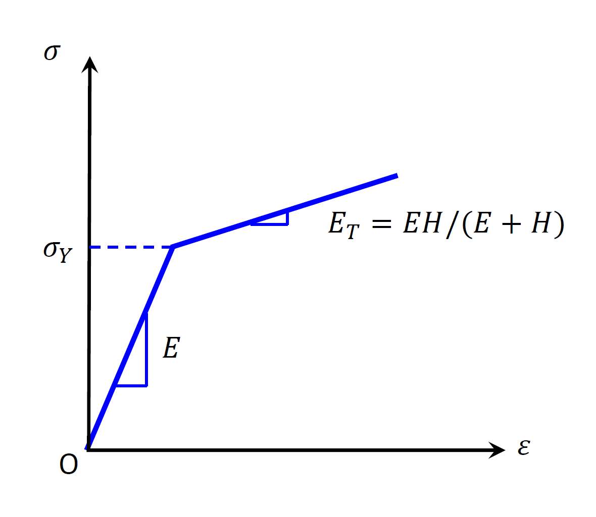
Figure 1: Von-Mises model in uniaxial loading.

Plastic Corrections

First, considering shear failure, partial differentiation of Equation (1) yields plastic strain

(7)\[ \epsilon^p_{ij} = {\lambda}^s {{\partial g^s}\over{\partial \sigma_{ij}}} = {\lambda}^s {{1.5(s_{ij}-\alpha_{ij})}\over{[ 1.5(s_{ij}-\alpha_{ij}) (s_{ij}-\alpha_{ij})]^{0.5}}}\]

apparently, \(\varepsilon^p_v = 0\), and \(e^p_{ij} = \epsilon^p_{ij}\).

The consistency condition of yield function

(8)\[ \Delta f^s(s^I_{ij} + \Delta s_{ij}, \alpha^I_{ij} + \Delta \alpha_{ij}) = 0\]

yields

(9)\[ {\lambda}^s = {{f^s(s^I_{ij}, \alpha^I_{ij})} \over {3G+H}}\]

von-mises Model Properties

Use the following keywords with the zone property (FLAC3D) or block zone property (3DEC) command and with the structure shell property (or liner/geogrid) command to set these properties of the von Mises model.

von-mises

bulk f

bulk modulus, \(K\)

modulus-plastic f

kinematic plastic (hardening) modulus, \(H\) (see Figure 2). The default value is zero. Be aware that this is not the elastoplastic tangent modulus, \(E_t\). The relationship between \(H\) and \(E_t\) is shown in Figure 2.

poisson f

Poisson’s ratio, \(\nu\)

shear f

shear modulus, \(G\)

strength-yield f

yield strength, \(\sigma_Y\)

young f

Young’s modulus, \(E\)

Notes

• Only one of the two options is required to define the elasticity: bulk modulus \(K\) and shear modulus \(G\), or Young’s modulus \(E\) and Poisson’s ratio \(\nu\). When choosing the latter, Young’s modulus \(E\) must be assigned in advance of Poisson’s ratio \(\nu\).

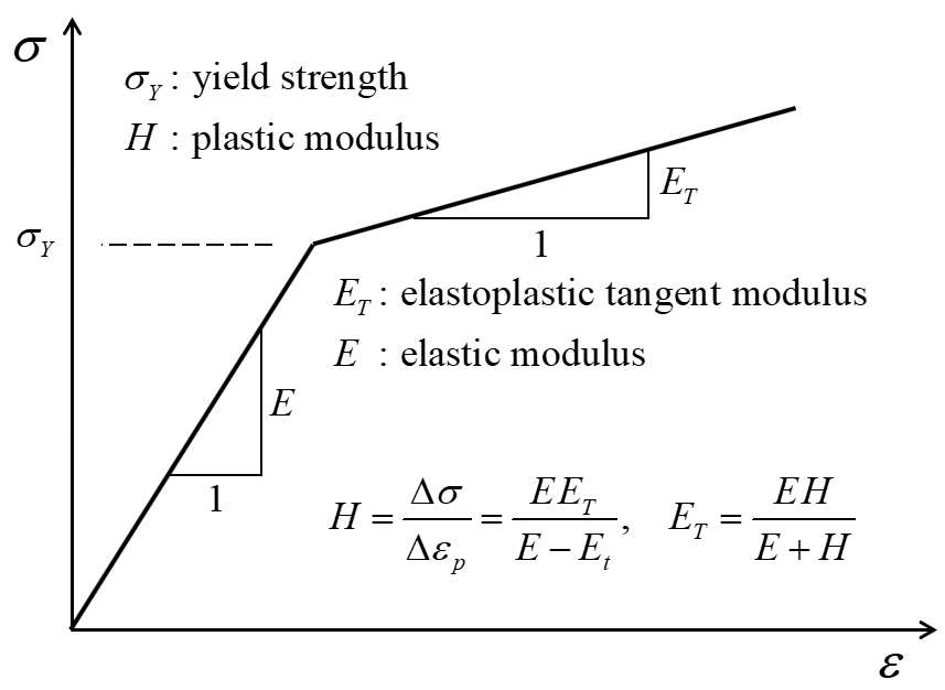
Figure 2: Behavior of von Mises model when subjected to uniaxial loading.