Beam-Type Structural Elements

The beam-type structural elements include beam elements and pile elements. The mechanical behavior of these elements can be divided into the structural response of the beam material itself, and the way the element interacts with the grid. The structural response of the beam material is common to all beam-type elements, and is described in this section. Specific behaviors that differ for each element type are described in the section for that type.

Like all structural elements (and unlike zones), individual beam-type elements are identified by their component-id numbers. Groups of beam-type elements are identified by id numbers. Individual structural nodes and links are also identified by component-id numbers. Nodes and links can also be selected by the id number of the elements they are attached to.

Mechanical Behavior

Beam behavior is typically idealized via two beam theories, which differ based on whether or not transverse shear deformation is considered. Euler-Bernoulli beam theory does not account for transverse shear deformation, while Timoshenko beam theory does account for such deformation. The kinematic assumptions of these two beam theories are similar to those for thin and thick plates as shown in Figure 1. The kinematic assumption in the Euler-Bernoulli beam theory is that a straight line oriented normal to the undeformed midsurface remains straight and normal to the deformed midsurface. This assumption is relaxed in the Timoshenko beam theory whereby a straight line oriented normal to the undeformed midsurface remains straight but not necessarily normal to the deformed midsurface. The relaxation of this constraint effectively lowers the stiffness of the beam. The effects of transverse shear deformation are negligible in long thin beams, for which the thickness is small relative to the length. These effects become important when modeling short thick beams. A beam can be considered to be short and thick if its length to thickness ratio is of the order of five or less, or if it has a small value of shear modulus \((G)\) relative to Young’s modulus \((E)\).[1]

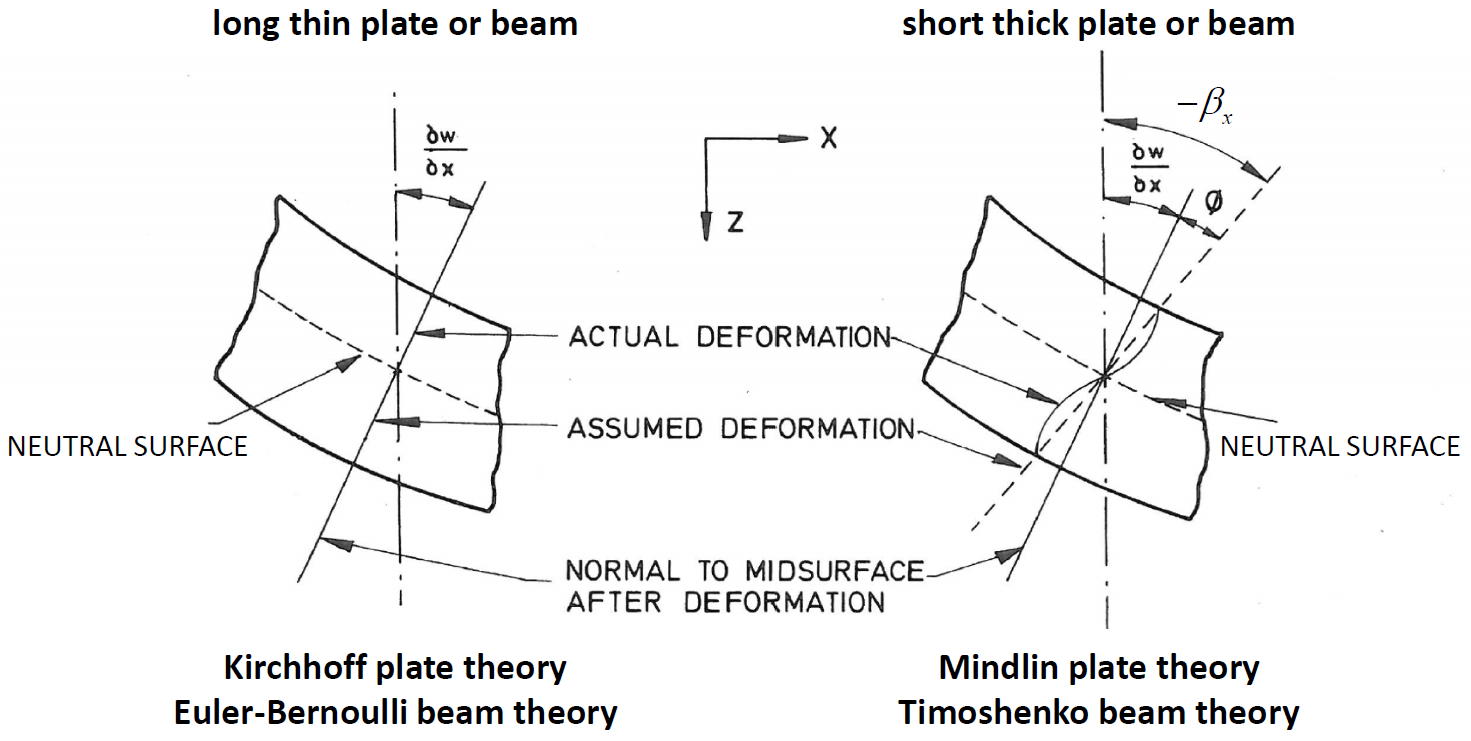
Figure 1: Cross-sectional deformation of beam illustrating the kinematic assumptions behind the beam theories. (From Fig. 4.1 of Hinton and Owen [1977])

Each beam-type structural element (beam or pile) is defined by its geometric and material properties. A beam-type element is assumed to be a straight segment of uniform bisymmetrical cross-sectional properties lying between two nodal points. An arbitrarily curved structural beam can be modeled as a curvilinear structure composed of a collection of beam elements. Each beam-type element behaves either as an elastic material with no failure limit or as a plastic material. One can specify a limiting plastic moment or introduce a plastic-hinge location (across which a discontinuity in rotation may develop) between beam elements (see Plastic Hinge Formation (with beam elements) ). Each beam-type element provides a different means of interacting with the grid (see Beam Structural Elements and Pile Structural Elements). The structural response of the beam is controlled by the constitutive model and the type of finite element. There are two finite elements available: an Euler-Bernoulli element (appropriate for modeling long thin beams), and a Timoshenko element (appropriate for modeling short thick beams). Plastic material behavior is supported only by the Euler-Bernoulli beam element and currently is available only in 3D. The general properties of these finite elements are described in Beam Finite Elements. The elements consider displacements resulting from uniform axial deformation, flexural deformation, and twisting deformation (3D ONLY). The 12 active degrees-of-freedom of the beam finite element are shown in Figure 2. For each generalized displacement (translation and rotation) shown in the figure, there is a corresponding generalized force (force and moment).

Each beam-type element has its own local coordinate system, shown in Figure 2. This system is used to specify both the cross-sectional moments of inertia and applied distributed loading. The beam element coordinate system is defined by the locations of its two nodal points (labeled 1 and 2 in the figures), and by the vector \(\bf Y\) such that:

1. the centroidal axis coincides with the \(x\)-axis;

2. the \(x\)-axis is directed from node-1 to node-2; and

3. the \(y\)-axis is aligned with the projection of \(\bf Y\) onto the cross-sectional plane (i.e., the plane whose normal is directed along the \(x\)-axis).

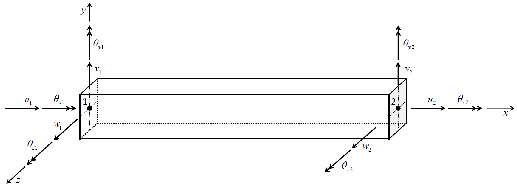
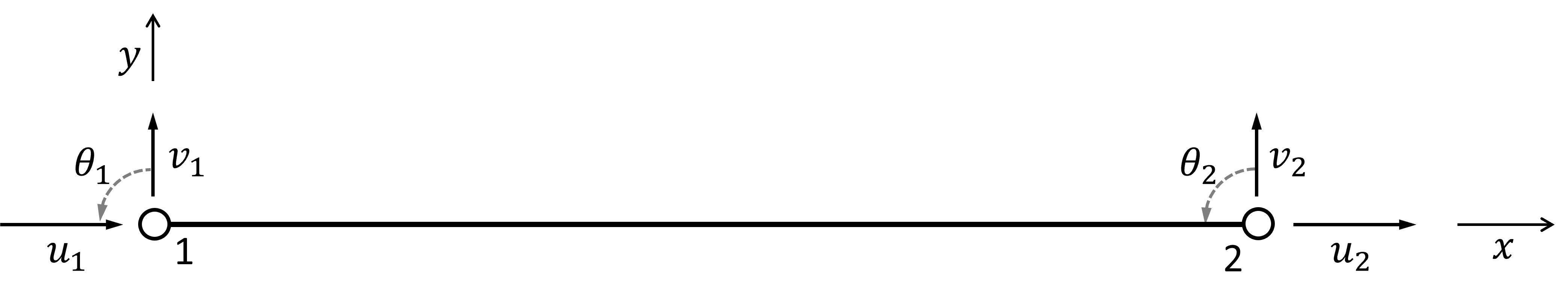
Figure 2: (Top) 3D beam-type element coordinate system and 12 degrees of freedom of the beam finite elements. (Bottom) 2D beam-type element coordinate system and 6 degrees of freedom

The beam element coordinate system can be modified with the structure beam property direction-y (or pile) command. (If \(\bf Y\) is not specified, or is parallel with the local \(x\)-axis, then \(\bf Y\) defaults to the global \(y\)- or \(x\)-direction, whichever is not parallel with the local \(x\)-axis.) The beam element coordinate system can be viewed with the Beam plot item and printed with the structure beam list system-local (or pile) command. The nodal connectivity can be printed with the structure beam list information (or pile) command.

The force-moment sign convention in Figure 3 provides a continuous description of axial-force, shear-force, twisting-moment, and bending-moment distributions across elements that make up a single beam-type structure (beam or pile). Note that the total force and total moment are reversed at end-1 of the element. This is done to insure that the force and moment distributions are continuous across elements. This will be the case if the set of elements making up the structure are oriented consistently, such that their local coordinate systems form a continuous description of the structure orientation. Such will be the case if the structure is created using the structure beam create or (or pile) command. The nodes of each element so created will be ordered such that the overall structure direction goes from the the first point to the second point.

The axial-force and twisting-moment distributions can be visualized with the Color By: Contour, and Value: Force or Moment, and Component: X setting of the beam and pile plot items. The shear-force and bending-moment distributions for bending in the \(xy\) and \(xz\) planes can be visualized with the Color By: Contour, and Value: Force or Moment, and Component: Y or Z settings of the beam and pile plot items. The magnitudes of the total shear force and total bending moment acting at the element ends can be visualized with the Color By:Contour, and Value: Force (shear) Magnitude and Moment (bending) Magnitude settings of the beam and pile plot items.

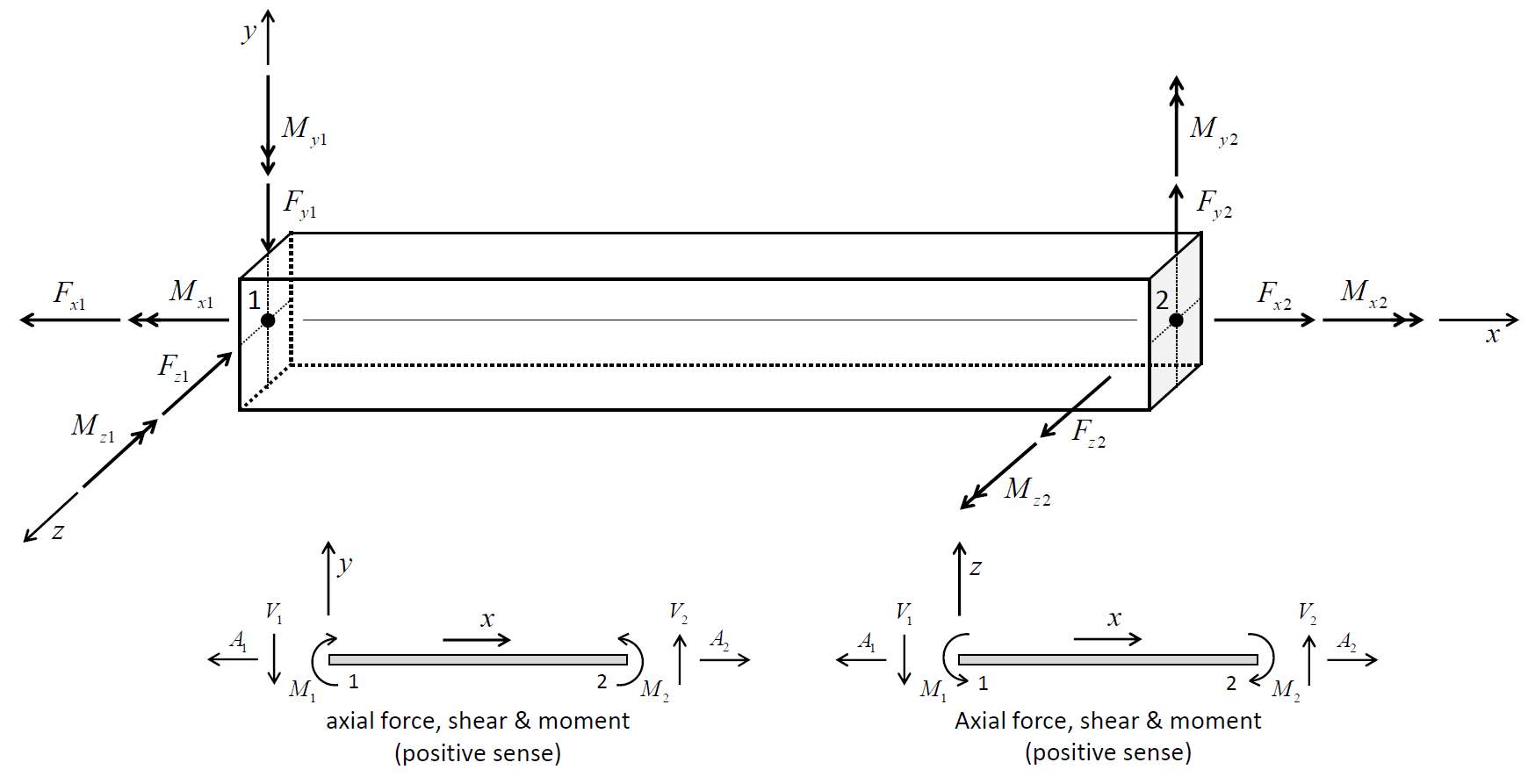
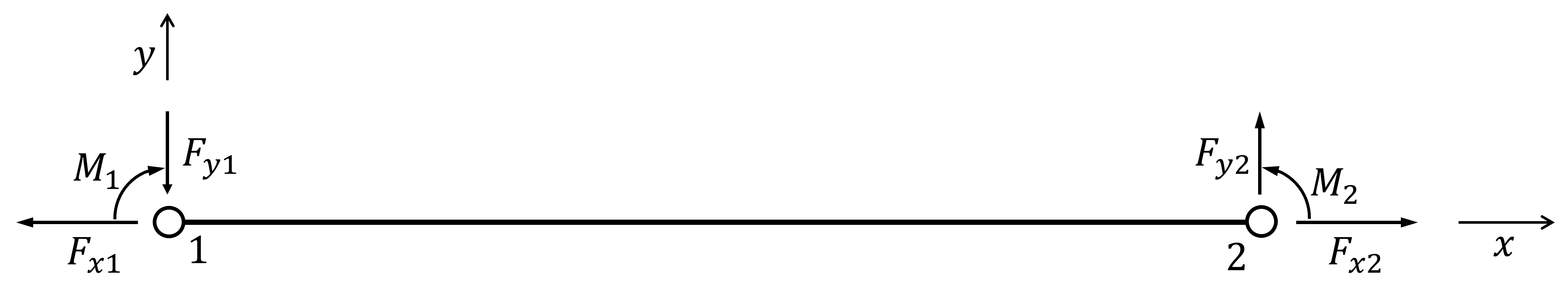
Figure 3: (Top) 3D Force-moment sign convention (Axes show beam-type element coordinate system, ends 1 and 2 correspond with order in nodal connectivity list, and all quantities are drawn acting in their positive sense). (Bottom) 2D Force-moment sign convention.

Response Quantities

Beam responses include force and moment vectors that act at the end of each beam element. These quantities can be expressed in the global system or in the beam element coordinate system. The beam responses can be accessed via FISH and

1. listed with the structure beam list force-node (or pile) command;

2. monitored with the structure beam history (or pile) command; and

3. visualized with the Beam and Pile plot items.

Beam Plasticity Plot Items

The stress, plastic state, and integration-point layout of beams with a plastic material model can be plotted with the Beam and Pile plot items as follows.

1. The {Contour Stress (plastic-max/min)} item colors each element with a plastic material model based on the maximum or minimum axial stress within the element by checking over all integration points.

2. The {Label Plastic Integration} item displays the integration-point layout for each element with a plastic material model. The layout is described by a set of three numbers labeled \(\{n_x,n_2,n_3\}\) where \(\{n_2,n_3\} = \{n_y,n_z\}\) for a beam with a rectangular cross section, and \(\{n_2,n_3\} = \{n_r,n_\theta\}\) for a beam with a circular cross section.

3. The {Label Plastic Yield} item shows the percentage of integration points that have yielded within each element with a plastic material model. The yield boundary is specified as a percentage between zero and one hundred, and the elements are colored to denote those that have not yielded and those whose yield percentage is above and below the yield boundary.

Beam-Type Properties

The properties of the beam material consist of constitutive model properties and the following 15 additional properties. If the beam has an elastic constitutive model, then \(E\) and \(\nu\) and the cross-sectional properties (\(A\), \(J\) and { \(I\) in 2D; \(I_y\) and \(I_z\) in 3D }) must be specified for the Euler-Bernoulli beam element, whereas these properties as well as the two shear coefficients (\(\kappa\) in 2D; \(\kappa_y\) and \(\kappa_z\) in 3D) must be specified for the Timoshenko beam element. If the beam has a plastic constitutive model, then the cross-sectional properties and shear coefficients need not be specified; instead, the cross-sectional shape and size must be specified as well as the constitutive model properties of \(E\) and \(\nu\). The cross-sectional shape is specified with the structure beam cmodel plastic-integration (or pile) command. The properties of \(E\) and \(\nu\) are specified with the young and poisson keywords of the structure beam property (or pile) command.

1. cross-sectional-area, cross-sectional area, \(A\) [L²]

2. density, mass density, \(\rho\) (optional — needed if dynamic mode or gravity is active) [M/L³]

3. direction-y, vector \(\bf Y\) whose projection onto the element cross-section defines the \(y\)-axis of the element coordinate system (optional — if not specified, \(\bf Y\) defaults to the global \(y\) or \(x\) direction, whichever is not parallel with the element \(x\) axis)

4. moi-y, moment of inertia with respect to element \(y\) axis; \(I_y\) [L⁴] (3D ONLY);

5. moi-z, moment of inertia with respect to element \(z\) axis; \(I_z\) [L⁴] (3D ONLY)

   moi, moment of inertia with respect to the element out-of-plane direction; \(I\) [L⁴] (2D ONLY)

6. plastic-moment, plastic moment capacity in Y and Z (out-of-plane in 2D) directions, \(M^P\) (optional — if not specified, then \(M^P\) is assumed to be infinite) [F\(\cdot\)L] If the plastic moment capacity was specified in Y and Z directions separately, then this value is the maximum of those components. If assigned, then the value is given to both the \(y\) and \(z\) components.

7. plastic-moment-y, plastic moment capacity in Y only, \(M_y^P\) (optional — if not specified, then \(M_y^P\) is assumed to be infinite) [F\(\cdot\)L] (3D ONLY)

8. plastic-moment-z, plastic moment capacity in Z only, \(M_z^P\) (optional — if not specified, then \(M_z^P\) is assumed to be infinite) [F\(\cdot\)L] (3D ONLY)

9. plastic-shear, plastic shear capacity in Y and Z (Y only in 2D) directions, \(V^P\) (optional — if not specified, then \(V^P\) is assumed to be infinite) [F] If the plastic shear capacity was specified in Y and Z directions separately, then this value is the maximum of those components. If assigned, then the value is given to both the \(y\) and \(z\) components.

10. plastic-shear-y, plastic shear capacity in Y only, \(V_y^P\) (optional — if not specified, then \(V_y^P\) is assumed to be infinite) [F] (3D ONLY)

11. plastic-shear-z, plastic shear capacity in Z only, \(V_z^P\) (optional — if not specified, then \(V_z^P\) is assumed to be infinite) [F] (3D ONLY)

12. shear-coefficient-y, shear coefficient for transverse shear deformation in the \(xy\)-plane[2] (Timoshenko beam only — see this discussion), \(\kappa_y\ (\kappa_y > 0)\)

13. shear-coefficient-z, shear coefficient for transverse shear deformation in the \(xz\)-plane (Timoshenko beam only), \(\kappa_z\ (\kappa_z > 0)\)

    shear-coefficient, shear coefficient for transverse shear deformation (Timoshenko beam only), \(\kappa\ (\kappa > 0)\) (2D ONLY)

14. thermal-expansion, thermal-expansion coefficient, \(\alpha_t\) [1/T]. Used with the thermal option to allow beam-type elements to experience strains arising from thermal expansion (as explained here).

15. torsion-constant, torsion constant, \(J\) [L⁴][3] (3D ONLY)

    spacing, out-of-plane distance btn. beam-type elements, \(S\) [L] (2D ONLY)

For the general beam-type element cross-section shown in Figure 4, the moment(s) of inertia (\(I\) in 2D; \(I_y\) and \(I_z\) in 3D) are defined in the element coordinate system \(xyz\) (\(z\) is the out-of-plane direction in 2D) by the integral(s)

(1)\[\begin{split}\left. \begin{array}{rl} I_y = \int_A z^2 \,dA \\ I_z = \int_A y^2 \,dA \end{array} \right\}3D\end{split}\]

\[\left. \begin{array}{rl} I = \int_A y^2 \,dA = \int_{-h/2}^{h/2} \int_{-b/2}^{b/2} y^2 \,dzdy = \displaystyle\frac{bh^3} {12} \end{array} \right.\text{ (2D)}\]

in which the two principal axes of the cross section are defined by the beam element \(y\)- and \(z\)-axes.

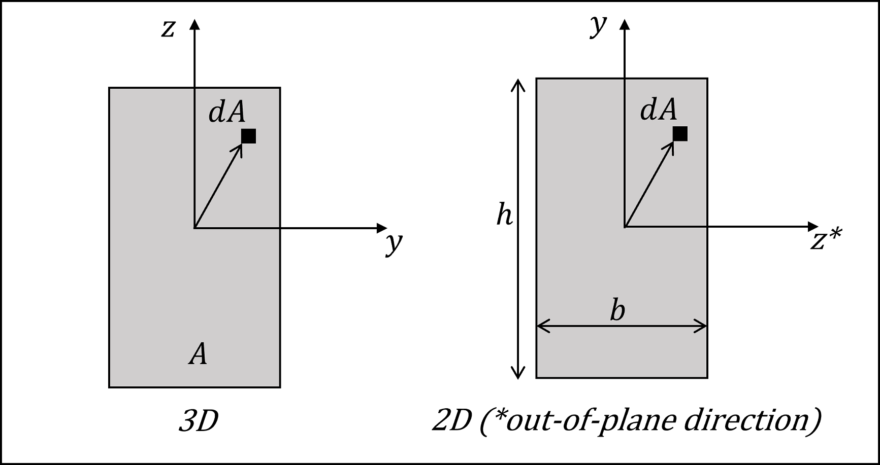
Figure 4: (Left) 3D Beam-type element cross-section in the element yz-plane. (Right) 2D Beam-type element cross-section in the element yz-plane.

Beam properties are easily calculated, or obtained from handbooks. For example, typical values for structural steel are 200 GPa for Young’s modulus, and 0.3 for Poisson’s ratio. For concrete, typical values are 25 to 35 GPa for Young’s modulus, 0.15 to 0.2 for Poisson’s ratio, and 2100 to 2400 kg/m³ for mass density. Composite systems, such as reinforced concrete, should be based on the transformed section.

If a plastic moment is specified, the value may be calculated as follows. Consider a flexural member of width, \(b\), and height, \(h\). If the member is composed of a material that behaves in an elastic-perfectly plastic manner, the elastic and plastic resisting moments can be computed. The moment necessary to produce yield stress, \(\sigma_y\), in the outer fibers is defined as the elastic moment, \(M^E\), and is calculated as

(2)\[M^E\ =\ \sigma_y\ {bh^2 \over{6}}\]

For yielding to occur throughout the section, the yield stress must act on the entire section, and the location of the resultant force on one-half of the section must be \(h/4\) from the neutral surface. The resisting moment, defined as the plastic moment, \(M^P\), is

(3)\[M^P\ =\ \sigma_y\ {bh^2 \over {4}}\]

The section at which the plastic moment occurs can continue to deform without inducing additional resistance after it reaches \(M^P\). The plastic-moment capacity limits the internal moment carried by each beam element.

In order to limit the moment that is transmitted between beam elements, the moment capacity at the nodes must also be restricted. The condition of increasing deformation with a limiting resisting moment that results in a discontinuity in the rotational motion is called a plastic hinge. Potential plastic-hinge locations can be defined by creating double nodes at each hinge location, adding a node-to-node link between these nodes, and then specifying appropriate link attachment conditions. If the limiting moment is reached at beam element connected by such a plastic hinge double-node, then a discontinuity in the rotational motion will develop. See Plastic Hinge Formation (with beam elements) for an example application of plastic hinges modeled with both single and double nodes.

The preceding discussion assumes a section that is symmetric about the neutral axis. However, if the section is not symmetric (for example, a T-section), or if the stress-strain relations for tension and compression differ appreciably (for example, reinforced concrete), the neutral axis shifts away from the fibers that yield first, and it is necessary to relocate the neutral axis before the resisting moment can be evaluated. The neutral axis may be found by integrating the stress profile over the section and solving for the location of the axis at which stress is zero. In some cases, the integral can be expressed in terms of one unknown (in which case, the solution may not be difficult). However, if the stress-strain relation for the material does not resemble an ideal elasto-plastic diagram, the solution may involve a number of trials. Nearly all texts on reinforced concrete or steel design provide procedures and examples for calculating plastic moments.

The present formulation in the program assumes that beam elements behave elastically until they reach the plastic moment. This assumption is reasonably valid for symmetric rolled-steel sections, because the difference between \(M^P\) and \(M^E\) is not large. However, for reinforced concrete, the plastic moment may be as much as an order of magnitude greater than the elastic moment.

Beam Elastic Constitutive Model

The beam elastic constitutive model updates the internal element forces by multiplying nodal displacement increments by an element stiffness matrix. The stiffness matrix is expressed in closed form, thus it is not necessary to perform numerical integration. There are two beam elements: the Euler-Bernoulli beam element that is appropriate for modeling long thin beams, and the Timoshenko beam element that is appropriate for modeling short thick beams. The stiffness matrices of both elements provide isotropic elastic material behavior (see Beam Mechanical Behavior and Beam Finite Elements). The cross-sectional properties must be specified for the Euler-Bernoulli beam element, and these properties as well as the two shear coefficients must be specified for the Timoshenko beam element (see Beam-Type Properties).

elastic Beam Model Properties

Use the following keywords with the structure beam property and structure pile property commands to set these properties of the beam isotropic elastic constitutive model.

elastic

young f

Young’s modulus, \(E\)

poisson f

Poisson’s ratio, \(\nu\)

Beam Plastic Constitutive Models (3D ONLY)

The beam plastic constitutive models update the internal element forces by integrating the internal stress over the beam volume using a numerical integration scheme. Stiffness matrices are not formed. The plasticity is induced by axial and bending deformations; twisting deformation induces an elastic response. The beam may have either a rectangular or circular cross section. Integration points are distributed throughout the volume of the beam elements as shown in Figures 5 and 6. An axial strain (\(\varepsilon_x\))is induced when the element is subjected to axial and bending deformation. The normal strains (\(\varepsilon_y\) and \(\varepsilon_z\)) satisfy plane-stress conditions. The transverse shear strains (\(\gamma_{xy}\) and \(\gamma_{xz}\)) are zero to satisfy the Euler-Bernoulli hypothesis that prohibits transverse shear deformation. The cross-sectional shear strain (\(\gamma_{yz}\)) is zero because the beam is symmetric about both principal cross-sectional axes. The only non-zero stress component is \(\sigma_x\). The total stress at each integration point (\(\sigma_x\)) is updated by the beam plastic constitutive model during each timestep. There are three beam plastic constitutive models, each of which is a one-dimensional version of the corresponding 3D model used by the zones. The constitutive models are von Mises, Mohr Coulomb, and Strain Softening/Hardening Mohr Coulomb. The first model is suitable for modeling steel beams, and the remaining two models are suitable for modeling concrete beams. Plasticity is provided only by the Euler-Bernoulli beam element. The formulation of nonlinear structural elements that provide beam plasticity is provided in Potyondy (2022).

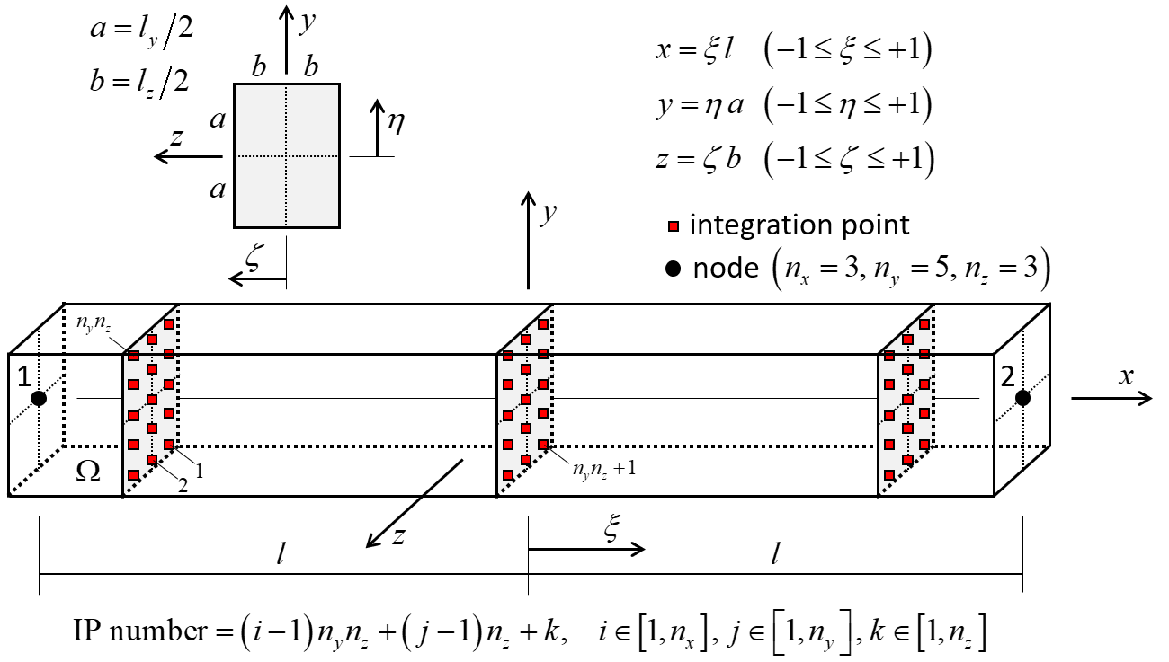
Figure 5: Beam element with rectangular cross section showing 45 integration points throughout the beam volume and integration-point numbering.

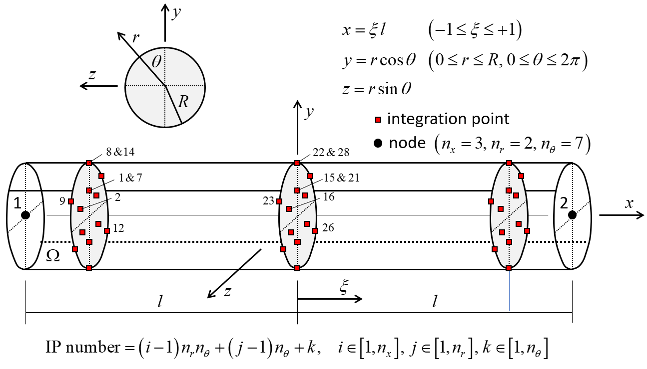
Figure 6: Beam element with circular cross section showing 42 integration points throughout the beam volume and integration-point numbering.

The integration-point layouts are shown in Figures 5 and 6. Gauss quadrature is used for integration along the beam length for both cross-sectional shapes. Gauss quadrature is used for integration over the cross-sectional area of the rectangular cross section, and closed composite Newton-Cotes quadrature of degree two is used for integration over the cross-sectional area of the circular cross section. The integration points of the rectangular cross section are offset from the element surface (see Figure 7), and thus, the scheme does not directly account for yielding on the surface as soon as it occurs.[4] The integration points of the circular cross section are on the element surface (see Figure 8), and thus, the scheme directly accounts for yielding on the surface as soon as it ocurs.

The expected accuracy of the integration scheme over the circular cross section can be compared with that of the integration scheme over the rectangular cross section by comparing the mean error obtained for the integration of stresses through the thickness of plates and shells when there are discontinuities in the stresses (see Figure 9). The rule that is circled and labeled “Simpson’s” is expected to correspond with the integration layout shown in Figure 8, and the rule that is circled and labeled “5-Gauss” is expected to correspond with the integration layout shown in Figure 7. Both of these layouts are expected to provide similar accuracy. Guidance for choosing the number of integration points through the thickness is given in this Figure.

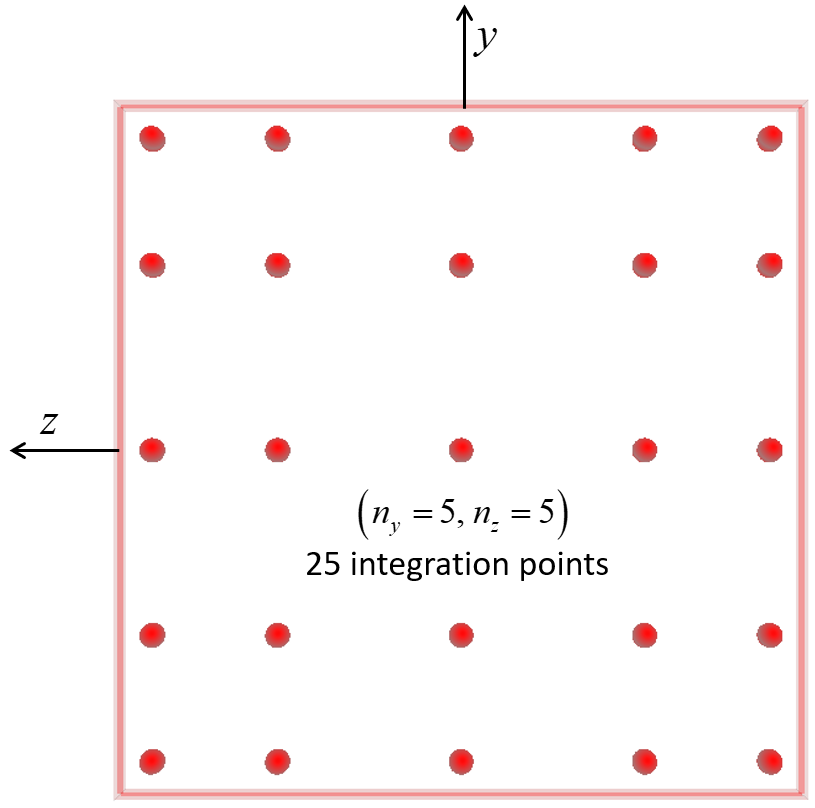
Figure 7: Beam element with rectangular cross section showing the layout of 25 integration points on the beam cross section.

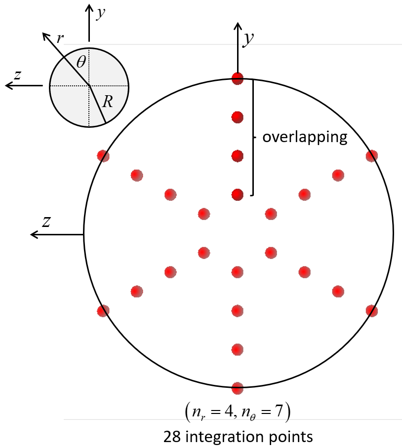
Figure 8: Beam element with circular cross section showing the layout of 28 integration points on the beam cross section. The integration points overlap along the upper half of the y axis.

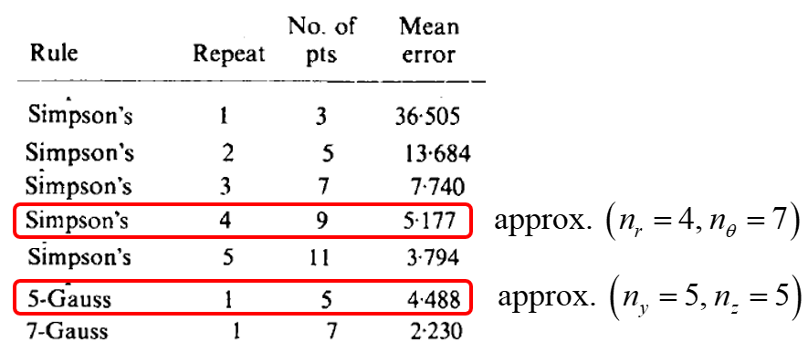
Figure 9: Mean error for integration of stress through the thickness of plates and shells when there are discontinuities in the stresses. (From Burgoyne and Crisfield [1990])

The constitutive model (and its properties, including the Poisson’s ratio) and the integration scheme (shape and size of the beam cross section and integration-point layout) must be specified for each plastic element with the structure beam cmodel assign and structure beam cmodel plastic-integration (or pile) commands. The plastic state, stress, and min/max axial stress are listed with the plastic-state, plastic-stress and plastic-stress-bounds keywords of the structure beam list (or pile) command. Histories of the axial stress at a specified integration point are sampled by the structure beam history ipstress (or pile) command. The stress, plastic state, and integration-point layout of beams with a plastic material model can be plotted with the Beam and Pile plot items (described here).

References

Burgoyne, C. J., and M. A. Crisfield. “Numerical Integration Strategy for Plates and Shells,” Int. J. Num. Meth. Engng., 29, 105–121 (1990).

Cirak, F. (2010) Course notes for “Plates and Shells: Theory and Computation,” University of Cambridge. [Accessed December 6, 2021 from http://www-g.eng.cam.ac.uk/csml/teaching as 4D9_handout2.pdf.]

Budynas, R. G., and A. M. Sadegh. Roark’s Formulas for Stress and Strain, Ninth Edition. McGraw-Hill Education (2020).

Cowper, G. R. “The Shear Coefficient in Timoshenko’s Beam Theory,” ASME Journal of Applied Mechanics, 33(2), 335–340 (1966).

Hinton, E., and D. R. J. Owen. Finite Element Programming. New York: John Wiley & Sons Inc. (1977).

Potyondy, D. “Nonlinear Structural Elements,” Itasca Consulting Group, Inc., Technical Memorandum 5-8121:22TM36 (September 9, 2022), Minneapolis, Minnesota (2022).

Endnotes

[1]

The closed-form solution for the tip deflection of a tip-loaded cantilever beam gives the ratio of Timoshenko to Euler-Bernoulli tip deflection (\(u^T/u^{EB} = 1 + {3 \over 5}(\frac{t}{L})^2\)) such that the difference in tip deflection reaches 2.4% when the length to thickness ratio reduces to five (Cirak, 2010). Budynas and Sadegh (2020) state that a beam can be considered to be short and thick if the span over depth ratio is 8 or less for metal beams of compact section, 15 or less for beams with relatively thin webs, and 24 or less for rectangular timber beams (which have a small value of \(G\) compared with \(E\)).

[2]

Commonly accepted shear coefficients are \(\kappa = 0.833\) for a solid rectangular cross section, and \(\kappa = 0.5\) for a thin-walled tube of circular cross section. More nearly exact shear coefficients appear in Cowper (1966). Note that as an element becomes more and more slender, \(\phi_y\) and \(\phi_z\) approach zero, so that flexural-stiffness coefficients in the Timoshenko beam stiffness matrix reduce to the flexural-stiffness coefficients for a Euler-Bernoulli beam, where transverse shear deformation is neglected. The flexural-stiffness coefficient that multiplies the nodal displacement in the \(z\)-direction to give the nodal force in the \(z\)-direction is \(12EI_y / (1+\phi_z)L^3\) with \(\phi_z = 12EI_y / \kappa_z G A L^2\). The flexural-stiffness coefficient that multiplies the nodal displacement in the \(y\)-direction to give the nodal force in the \(y\)-direction is \(12EI_z / (1+\phi_y)L^3\) with \(\phi_y = 12EI_z / \kappa_y G A L^2\).

[3]

The \(\theta_x\) degrees of freedom account for twist about the \(x\) axis, for which the stiffness coefficient is \(GJ / L\), where the torsion constant \((J)\) is a property of the shape and size of the cross section. Only for a circular cross section, either solid or a tube, does \(J\) become equal to the polar moment of inertia of the cross section. For thin-walled open cross sections, such as those of standard I beams and channels, \(J\) is a small fraction of the polar moment of inertia. Values of \(J\) for various cross-sectional shapes are given in Budynas and Sadegh (2020).

[4]

The rationale for the use of Gauss quadrature to integrate through the thickness of the shell elements is presented in the text associated with the figure shown in Shell-Type Structural Elements. It is expected that the same considerations apply to integrating over the rectangular cross section of the beam.