Geogrid Structural Elements (3D Only)
Note that geogrid structural elements are based on the Shell-Type Structural Element and share the underlying formulation and implementation.
Mechanical Behavior
The mechanical behavior of each geogrid element can be divided into the structural response of the geogrid material itself (see Shell-Type Mechanical Behavior) and the way in which the geogrid element interacts with the model grid. By default, geogrid elements are assigned the CST plane-stress element that resists membrane but does not resist bending loading (see Shell Finite Elements). A membrane structure can be modeled as a collection of geogrid elements. The geogrid behaves as an isotropic or orthotropic, linear elastic material with no failure limit. A shear-directed (in the tangent plane to the geogrid surface) frictional interaction occurs between the geogrid and the model grid, and the geogrid is slaved to the grid motion in the normal direction. The geogrid can be thought of as the two-dimensional analog of a one-dimensional cable. Geogrids are used to model flexible membranes whose shear interaction with the soil are important, such as geotextiles and geogrids.
The orientation of the node-local system for all nodes used by geogrid elements is set automatically at the start of a set of cycles (or when the model cycle 0 command is executed), such that the \(z\)-axis is aligned with the average normal direction of all geogrid elements using the node, and the \(xy\)-axes are arbitrarily oriented in the geogrid tangent plane (see Figure 2).
A geogrid is embedded in the interior of the model grid. The behavior at the geogrid-soil interface is summarized in Figures 1 to 2. The stresses acting on the geogrid are shown in Figure 1. These stresses, consisting of an effective confining stress, \(\sigma_m\), and a total shear stress, \(\tau\), are balanced by the membrane stresses that develop within the geogrid itself. These membrane stress resultants (see Stresses in Shells) are denoted by \(\bar N\) in Figure 1. The interface behavior is represented numerically at each geogrid node by a rigid attachment in the normal direction and a spring-slider in the tangent plane to the geogrid surface. The orientation of the spring-slider changes in response to relative shear displacement \({\bf u}_s\) between the geogrid and the host medium, as shown in Figure 2. The fact that there is only a single spring slider at each node makes the geogrid behave in a fashion similar to a coarse mesh of cross-linked bars. The spring-slider carries the total shear force acting over the tributary area on both sides of the geogrid surface. Also, the effective confining stress is assumed to be acting equally on both sides of the geogrid surface.
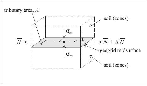
Figure 1: Stresses acting on the geogrid elements surrounding a node
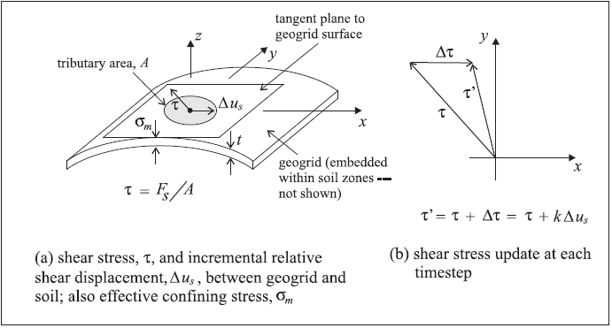
Figure 2: Idealization of interface behavior at a geogrid node
The normal behavior of the geogrid-soil interface is described below. The shear behavior of the geogrid-soil interface (see Figure 3) is cohesive and frictional in nature, and is controlled by the coupling spring properties of (1) stiffness per unit area, \(k\), (2) cohesive strength, \(c\), (3) friction angle, \(\phi\), and (4) effective confining stress, \(\sigma_m\). Note that the coupling-spring properties associated with each geogrid element are averaged at geogrid nodes.
The effective confining stress, \(\sigma_m\), acts perpendicular to the geogrid surface, and is computed at each geogrid node, based on the stress acting in the single zone to which the node is linked. Denote the geogrid surface normal direction as \(z\). The value of \(\sigma_m\) is taken as
where: \(p\) = pore pressure
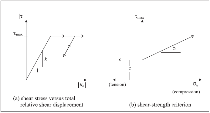
Figure 3: Shear-directional interface behavior for geogrid elements
In computing the relative displacement at the geogrid-soil interface, an interpolation scheme is used to calculate the grid displacement, based on the displacement field in the zone to which the node is linked. The interpolation scheme uses weighting factors that are determined by the distance to each of the zone gridpoints. The same interpolation scheme is used to apply forces developed in the geogrid-soil interface back to the gridpoints of the zone.
As explained above, an interpolated estimate of grid velocity is made at each geogrid node. The velocity normal to the geogrid surface is transferred directly to the node (i.e., the geogrid node is slaved to the grid motion in the normal direction). The node exerts no normal force on the grid if all the geogrid elements that share the node are coplanar; however, if they are not coplanar, then a proportion of their membrane force will act in the normal direction. This net force acts both on the grid and on the geogrid node (in opposite directions). Thus, an initially flat geogrid can sustain normal loading if it is allowed finite deflection, using the large-strain solution mode. This normal force is transferred to the gridpoints of the single zone to which the node is attached. The attachment is to only one zone on one side of the geogrid surface, and this side may not correspond with the side going into compression. There is no provision for the formation or tracking of gaps between the geogrid and the soil (i.e., the geogrid is assumed to be fully embedded within the soil at all times).
Geogrids support large-strain sliding (by setting the slide property to on), whereby the interpolation locations (used by the geogrid nodes to transfer forces and velocities to and from the zones — see Structural Element Links) will migrate through the grid when running in large-strain mode. This allows one to calculate the large-strain, post-failure behavior of a geogrid, whereby substantial sliding between the geogrid nodes and the zones occurs. If a geogrid node moves out of all zones, then a connection with the zones will not be reestablished if the node is later moved back into zones; however, the connection remains intact as the geogrid nodes slide between zones.
Response Quantities
Geogrid responses include stresses in the geogrid itself, as well as stress, displacement and yield state in the coupling springs. Additional coupling-spring information includes the current loading direction and the effective confining stress. The geogrid responses can be accessed via FISH, and
listed with the
structure geogrid listcommand,monitored with the
structure geogrid historycommand, andplotted with the Geogrid plot item.
Refer to Shell-Type Response Quantities for a summary of the commands that support recovery of stresses acting in the geogrid itself.
Properties
Each geogrid element has 5 properties in addition to those common to all shell-type elements described in Shell-Type Properties. These five properties control the shear behavior of the geogrid-soil interface.
coupling-cohesion, coupling spring cohesion (stress units), \(c\) [F/L2]coupling-friction, coupling spring friction angle, \(\phi\) (degrees)coupling-stiffness, coupling spring stiffness per unit area, \(k\) [F/L3]slide, large-strain sliding flag (default:off)slide-tolerance, large-strain sliding tolerance
Examples
Simple examples are given to illustrate the use of geogrids. This list is incomplete; a complete list of examples that use geogrid elements is available in Structural Geogrid Examples.
Commands & FISH
| Was this helpful? ... | Itasca Software © 2024, Itasca | Updated: Apr 02, 2024 |
