Liner Structural Elements (2D)
Note that liner structural elements are based on the Beam-Type Structural Element and share the underlying formulation and implementation.
Mechanical Behavior
Single-Sided Liner-Grid Interaction
The mechanical behavior of each liner element can be divided into the structural response of the liner material itself (see Beam-Type Mechanical Behavior), and the way in which the liner element interacts with the model grid. By default, liner elements are assigned as beam finite elements (see Beam Finite Elements). A physical liner can be modeled as a collection of liner elements that are attached to the surface of the model grid. In addition to providing the structural behavior of a beam, a shear-directed (in the tangent plane to the liner surface) frictional interaction occurs between the liner and the model grid. Also, in the normal direction, both compressive and tensile forces can be carried, and the liner may break free from (and subsequently come back into contact with) the grid. Liners are used to model thin liners for which both normal-directed compressive/tensile interaction and shear-directed frictional interaction with the host medium occurs, such as shotcrete-lined tunnels or retaining walls.
The orientation of the node-local system for all nodes used by liner elements is set automatically at the start of a set of cycles (or when the model cycle 0 command is executed) such that the \(y\)-axis is aligned with the average normal direction of all liner elements using the node, and the \(x\)-axis are arbitrarily oriented in the liner element tangent plane (see Figure 2 (a)). Additionally, if the liner elements are attached to a zone face, the \(y\)-axis will be aligned to the normal direction of the zone face.
Note
Beam, cable, pile and rockbolt elements in 2D adhere to a plane-stress formulation. Since liner elements represent a structure that is continuous in the direction perpendicular to the analysis plane (e.g. a concrete tunnel lining), the value for \(E\) is automatically divided by \((1-\nu^2)\) to account for plane-strain conditions.
A liner is attached to the surface of the model grid. The behavior at the liner-zone interface is summarized in Figures Figures #liner2d-stresses and 2. The forces acting on the liner (per unit length, \(L\)) are shown in Figure 1. These forces, consisting of a normal force, \(F_n\), and a shear force, \(F_s\), are balanced by forces that develop within the liner itself. The interface behavior is represented numerically at each liner node by a linear spring with finite tensile strength in the normal direction, and a spring-slider in the tangent plane to the liner surface. The orientation of the spring-slider changes in response to relative shear displacement \({\bf u}_s\) between the liner and the host medium, as shown in Figure 2. (Note that the liner is drawn below the zones in Figure 1 and above the zones in Figure 2.)
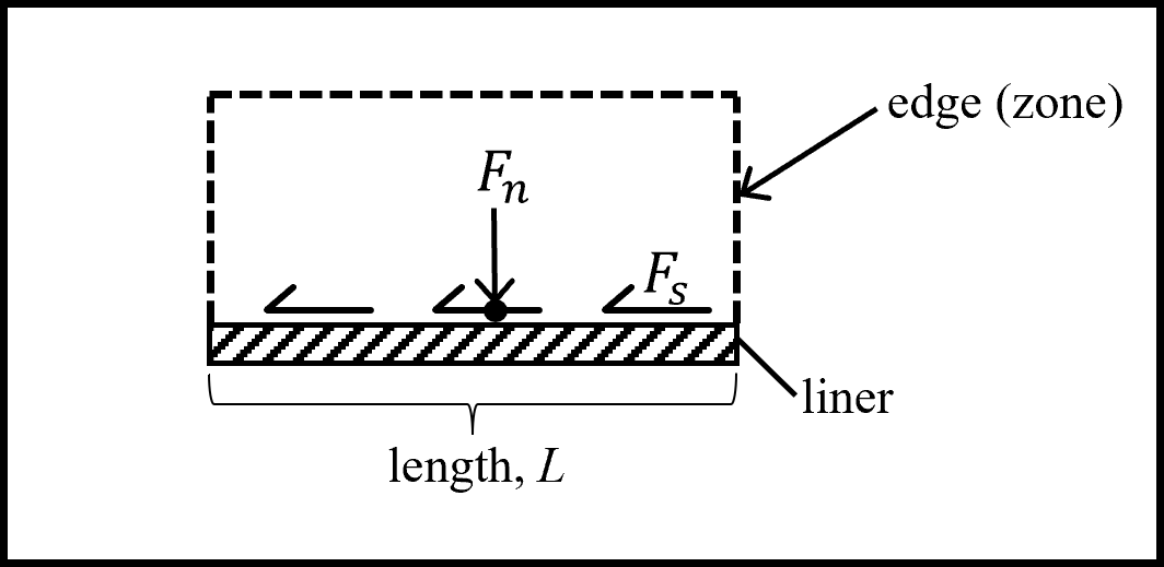
Figure 1: Forces acting on the liner elements surrounding a node
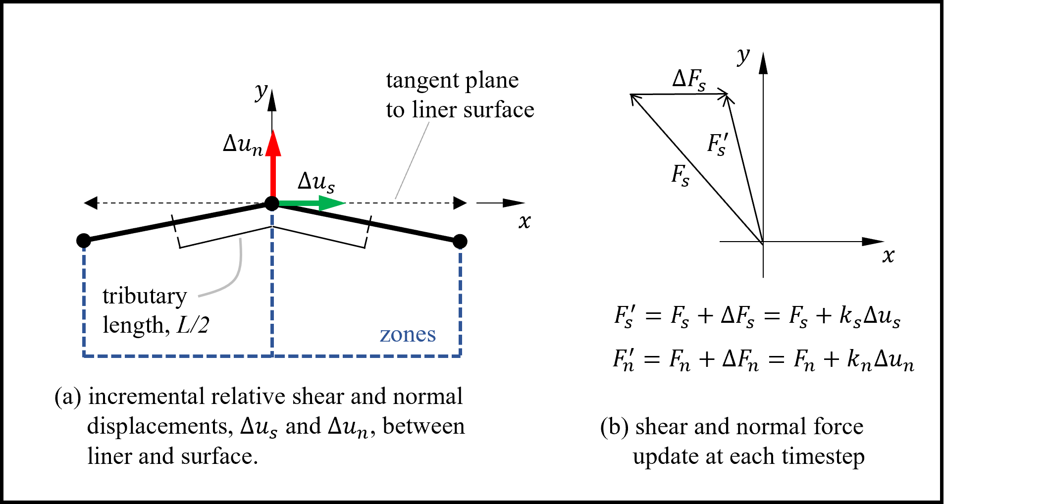
Figure 2: Idealization of interface behavior at a liner node
The normal behavior of the liner-zone interface (see Figure 3) is controlled by the normal coupling spring properties of (1) stiffness per unit area, \(k_n\), and (2) tensile strength, \(f_t\). The shear behavior of the liner-zone interface (see Figure 4) is cohesive and frictional in nature, and is controlled by the shear coupling spring properties of (1) stiffness per unit area, \(k_s\), (2) cohesive strength, \(c\), (3) residual cohesive strength, \(c_r\), and (4) friction angle, \(\phi\), and by the interface normal stress, \(\sigma_n\). If the liner fails in tension, then the effective cohesion drops from \(c\) to \(c_r\), and the tensile strength is set to zero. The total relative normal displacement, \(u_n\), continues to be tracked such that compressive normal stresses will again develop when the gap closes. Note that the coupling spring properties associated with each liner element are averaged at liner nodes.
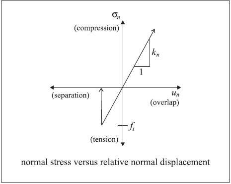
Figure 3: Normal-directional interface behavior for liner elements
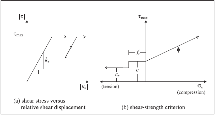
Figure 4: Shear-directional interface behavior for liner elements
In computing the relative displacement at the liner-zone interface, an interpolation scheme is used to calculate the grid displacement, based on the displacement field in the zone to which the node is linked. The interpolation scheme uses weighting factors that are determined by the distance to each of the zone gridpoints. The same interpolation scheme is used to apply forces developed in the liner-zone interface back to the gridpoints of the zone.
Liners support large-strain sliding (by setting the slide property to on), whereby the interpolation locations (used by the liner nodes to transfer forces and velocities to and from the zones — see Structural Element Links) will migrate through the grid when running in large-strain mode. This allows one to calculate the large-strain, post-failure behavior of a liner, whereby substantial sliding between the liner nodes and the zones occurs. At each liner node, if large-strain sliding is on and the tensile stress exceeds the interface tensile strength, then the link that joins this liner node to a zone surface will be deleted; however, if this node later comes back into contact with any zone face, the connection will be reestablished (via a new link with appropriate liner properties).
Embedded Liner Behavior
The liner structural element can also be made to interact with zones on both sides of the liner. Additional coupling springs are added to the embedded liner for this capability. (The default liner only provides a single link on each node, whereas the embedded liner provides two links on each node.) Independent properties are specified on each side of the embedded liner (side 1 and side 2). The embedded liner mechanical behavior is similar to the default liner behavior described above, except that the zone-liner interface is active on both sides of the embedded liner.
Response Quantities
Liner responses include force and moment acting on the liner itself, as well as stress, displacement, yield state and loading direction in both the normal and shear coupling springs. The liner responses can be accessed via FISH, and
listed with the
structure liner listcommand,monitored with the
structure liner historycommand, andplotted with the Liner plot item.
The sign convention used to plot force and moment distributions along the liner axis is described in force-moment sign convention.
Embedded Liner Response Quantities
Embedded liner response quantities are similar to the default liner response quantities described above, except that links or associated quantities can be associated with side 2 as well as side 1, or can be specified with structure liner history command.
The Liner plot item may be colored differently on each side to help identify side 1 and side 2.
Properties
Each liner element has 9 properties in addition to those common to all beam-type elements described in Beam-Type Properties. These properties control the shear and normal behavior of the liner-soil/rock interface.
coupling-cohesion-shear, shear coupling spring cohesion, \(c\) [F/L]coupling-cohesion-shear-2, shear coupling spring cohesion on side 2, \(c\) [F/L]coupling-cohesion-shear-residual, shear coupling spring residual cohesion, \(c_r\) [F/L]coupling-cohesion-shear-residual-2, shear coupling spring residual cohesion on side 2, \(c_r\) [F/L]coupling-friction-shear, shear coupling spring friction angle, \(\phi\) (degrees)coupling-friction-shear-2, shear coupling spring friction angle on side 2, \(\phi\) (degrees)coupling-stiffness-normal, normal coupling spring stiffness per unit length, \(k_n\) [F/L]coupling-stiffness-normal-2, normal coupling spring stiffness per unit length on side 2, \(k_n\) [F/L]coupling-stiffness-shear, shear coupling spring stiffness per unit length, \(k_s\) [F/L]coupling-stiffness-shear-2, shear coupling spring stiffness per unit length on side 2, \(k_s\) [F/L]coupling-yield-normal, normal coupling spring tensile strength, \(f_t\) [F/L]coupling-yield-normal-2, normal coupling spring tensile strength on side 2, \(f_t\) [F/L]effective, effective stress flag (default:on). Ifoff, then pore pressures are not removed from the stress normal to the liner when determining shear failure limits.slide, large-strain sliding flag (default:off)slide-tolerance, large-strain sliding tolerance
The properties can be divided into strength (\(f_t\), \(c\), \(c_r\), \(\phi\)) and stiffness (\(k_n\), \(k_s\)) properties. Choice of appropriate strength properties should be relatively straightforward, as they correspond with measurable macroscopic strength properties of the real physical system. Choice of the stiffness properties is more complex and will be discussed below (refer to Interfaces for a more detailed discussion).
Typically, we want the liner-zone interface to be stiff compared to the surrounding material, but able to slip and perhaps open in response to the anticipated loading. For this situation, we simply need to provide a means by which the liner elements can slide and/or open relative to the zone surfaces. The strength properties are important, but the elastic stiffnesses are not. It is recommended that the lowest stiffness consistent with small interface deformation be used. A good rule-of-thumb is that \(k_n\) and \(k_s\) be set to ten times the equivalent stiffness of the stiffest neighboring zone. The apparent stiffness (expressed in stress-per-distance units) of a zone in the direction normal to the surface is
where: |
\(K\) and \(G\) |
= |
the bulk and shear modulus, respectively; and |
\(\Delta z_{\rm min}\) |
= |
the smallest dimension of an adjoining zone in the normal direction. |
The \({\mathrm{max}} [ \ ]\) notation indicates that the maximum value over all zones adjacent to the liner is to be used (e.g., there may be several materials adjoining the liner). Note that Eq. (1) strictly applies only to a planar surface subjected to normal penetration. If the surface is curved, as is the case surrounding a circular excavation, the apparent stiffness should be increased by a factor of 10 to 100. For a particular problem, it is recommended that one confirm that the interface deformation (i.e., the displacement in the coupling springs) is small relative to the zone deformation. (The coupling spring displacements are obtained via the structure liner list coupling-normal and structure liner list coupling-shear commands; the zone displacement is obtained via the zone gridpoint list displacement command.)
Example Applications
Simple examples are given to illustrate the use of a liner.
A complete list of examples that use liners is available in Structural Liner Examples.
Commands & FISH
⇐
struct.liner.shear.stress |
Lined Circular Tunnel in an Elastic Medium with Anisotropic Stresses ⇒
| Was this helpful? ... | Itasca Software © 2024, Itasca | Updated: Apr 02, 2024 |
