Shell-Type Structural Elements (3D Only)

The shell-type structural elements include shell elements, geogrid elements and liner elements. The mechanical behavior of these elements can be divided into the structural response of the shell material itself, and the way the element interacts with the grid. The structural response of the shell material is common to all shell-type elements, and is described in this section. Specific behaviors that differ for each element type are described in the section for that type.

Like all structural elements (and unlike zones), individual shell-type elements are identified by their component-id numbers. Groups of shell-type elements are identified by id numbers. Individual structural nodes and links are also identified by component-id numbers. Nodes and links can also be selected by the id number of the elements they are attached to.

Mechanical Behavior

Each shell-type structural element (shell, geogrid, or liner) is defined by its geometric and material properties. A shell-type element is assumed to be a triangle of uniform thickness lying between three nodal points. An arbitrarily curved structural shell can be modeled as a faceted surface composed of a collection of shell-type elements. Each shell-type element behaves either as an elastic material with no failure limit or as a plastic material. One can introduce a plastic-hinge line (across which a discontinuity in rotation may develop) along the edges between shell-type elements, using the same double-node procedure as applied to beams (see Plastic Hinge Formation (with shell elements)). Each shell-type element provides a different means of interacting with the grid (see Shell Structural Elements, Geogrid Structural Elements, and Liner Structural Elements). The structural response of the shell is controlled by the constitutive model and the type of finite element. There are five finite elements available: 2 membrane elements, 1 plate-bending element and 2 shell elements. The general properties of these finite elements are described in Shell Finite Elements. Because these are all thin-shell finite elements, shell-type elements are suitable for modeling thin-shell structures in which the displacements caused by transverse-shearing deformations can be neglected. Thick-shell structures should be modeled with zones.

There are three coordinate systems associated with each shell-type element. A material coordinate system is used to specify orthotropic and anisotropic elastic material properties, and a surface coordinate system (providing a continuous description of the shell mid-surface spanning adjacent shell-type elements) is used to recover stresses — see Stresses in Shells. The element coordinate system is defined by the locations of its three nodal points (labeled 1, 2 and 3 in Figure 1) such that

1. the element lies in the \(xy\)-plane,

2. the \(x\)-axis is directed from node-1 to node-2, and

3. the \(z\)-axis is normal to the element plane and positive on the “outside” of the shell surface. (The two sides of each element are designated as outside and inside.)

The element coordinate system cannot be modified.

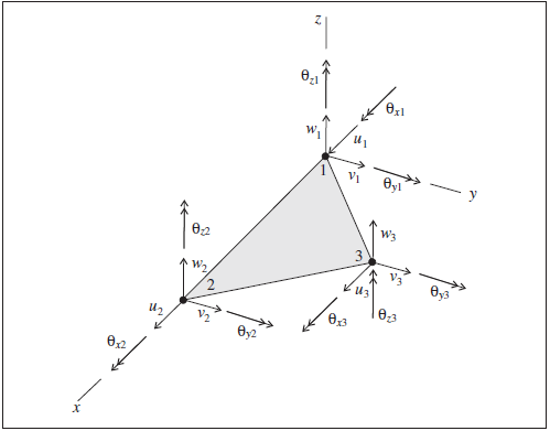
Figure 1: Shell-type element coordinate system and 18 degrees of freedom of the shell finite elements (The CST element does not utilize the rotations about the \(z\) axis.)

Response Quantities

Stress quantities, which include stress resultants and stresses acting in the shell, can be recovered for all shell-type elements (see Stress Recovery Procedure). The stress resultants are expressed in a surface coordinate system that provides a continuous description of the shell mid-surface spanning adjacent shell-type elements. The stresses for an elastic material are expressed in the global coordinate system, while the stresses for a plastic material are expressed in the surface coordinate system. The stress quantities can be accessed via FISH, and

1. listed with the structure shell list resultants, structure shell list stress, structure shell list stress-bounds, structure shell list stress-principal, structure shell list plastic-state and structure shell list plastic-stress commands, or the equivalent for geogrid or liner elements,

2. monitored with the structure shell history (or liner/geogrid) command, and

3. plotted with the Shell, Geogrid, or Liner plot items.

The surface coordinate system is established, and the stress resultants are recovered, with the structure shell recover (or liner/geogrid) command. This information is stored with the model and is accessible via FISH. The field variations are displayed as contours using the {Structural Element:Shell} (or liner/geogrid) plot item. If the {Use Engine Data} box is checked, then the recovered information (which is stored within the computational model — or engine) is displayed. If the {Use Engine Data} box is not checked, then the recovery process is triggered on the fly by the plot item, and in particular, the surface system is regenerated by projecting a surface-X vector (specified in the {SurfX} box) on the shell-type elements in the plot. To insure that the manually recovered data is plotted, one should check the {Use Engine Data} box.

Shell Plasticity Plot Items

The stresses, plastic state and integration-point layout of shells with a plastic material model can be plotted with the Shell, Liner and Geogrid plot items as follows.

1. The {Contour Stress (plastic-max/min)} item colors each element with a plastic material model based on the maximum or minimum stress within the element. The 2D plane-stress principal values (\(\sigma_1\) and \(\sigma_2\)) are found for the stress at the centroid of each layer of integration points, and the largest and smallest of these values over all layers are taken as the maximum and minimum stresses. The maximum and minimum stress within an element with an elastic material model can be displayed with the {Contour Stress (elastic-max/min} plot item. See the structure shell list stress-bounds (or liner/geogrid) command for a detailed description of how these stresses are computed.

2. The {Contour Stress (plastic)} item displays the specified component (\(\sigma_{xx}\), \(\sigma_{yy}\), or \(\sigma_{xy}\)) of the stress in the surface coordinate system at the centroid of the integration point layer nearest to the specified depth (where depth equals depth factor times one-half thickness) of each element with a plastic material model. The surface coordinate system must be set for all nodes used by the shells in the plot. The shells for which this is not the case have their stress compenent displayed as zero — in the current implementation a warning message is displayed and the plot it deactivated. The surface coordinate system is set via the structure shell recover surface (or liner/geogrid) command.

3. The {Label Plastic Integration} item displays the integration-point layout (number of integration points through the thickness and over the element area) for each element with a plastic material model.

4. The {Label Plastic State} item displays the yield state (never yielded, tension-p, shear-p, etc.) for the specified integration point on the layer of integration points nearest to the specified depth (where depth equals depth factor times one-half thickness) for each element with a plastic material model.

5. The {Label Plastic Yield} item shows the percentage of integration points that have yielded within each element with a plastic material model. The yield boundary is specified as a percentage between zero and one hundred, and the elements are colored to denote those that have not yielded and those whose yield percentage is above and below the yield boundary.

Shell-Type Properties

The properties of the shell material consist of constitutive model properties and the following three additional properties.

1. density, mass density, \(\rho\) [M/L³] (needed if dynamic mode or gravity is active)

2. thermal-expansion, thermal-expansion coefficient, \(\alpha_t\) [1/T]. Used with the thermal option to allow shell-type elements to experience strains arising from thermal expansion (as explained here).

3. thickness, shell thickness, \(t\) [L]

Shell Elastic Constitutive Models

The elastic constitutive models update the internal element forces by multiplying nodal displacement increments by an element stiffness matrix. The stiffness matrix is expressed in closed form, and thus, it is not necessary to perform numerical integration. The shell-type elements model general shell behavior as a superposition of membrane and bending actions via the five 3-noded triangular finite elements described in Shell Finite Elements. The material properties of the three shell elastic constitutive models are expressed via the membrane and bending material-rigidity matrices

(1)\[\begin{split}\begin{split} \big[ {\mathbf D}_m \big] &= \int_{-{t_m/2}}^{+{t_m/2}} \big[ {\mathbf E}_m \big]\,dz = t_m\,\big[ {\mathbf E}_m \big] \\[12pt] \big[ {\mathbf D}_b \big] &= \int_{-{t_b/2}}^{+{t_b/2}} \big[ {\mathbf E}_b]\,z^2dz = {{t_b^3} \over {12}} \big[ {\mathbf E}_b \big] \end{split}\end{split}\]

respectively, where \(t_m\) and \(t_b\) are the shell thicknesses used for membrane and bending actions, respectively, and \(\big[ {\mathbf{E}_m} \big]\) and \(\big[ {\mathbf{E}_b} \big]\) are material-stiffness matrices that relate stresses to strains via the constitutive relations

(2)\[\begin{split}\begin{split} \begin{Bmatrix} \boldsymbol\sigma_m \end{Bmatrix} &= {\begin{Bmatrix} \sigma_x \\ \sigma_y \\ \tau_{xy} \end{Bmatrix}}_m = \begin{bmatrix} {\bf E}_m \end{bmatrix} \begin{Bmatrix} \boldsymbol\varepsilon \end{Bmatrix} = \begin{bmatrix} c_{11}^m & c_{12}^m & c_{13}^m \\ & c_{22}^m & c_{23}^m \\ sym. & & c_{33}^m \end{bmatrix} \begin{Bmatrix} \varepsilon_x \\ \varepsilon_y \\ \gamma_{xy} \end{Bmatrix} \\[12pt] \begin{Bmatrix} \boldsymbol\sigma_b \end{Bmatrix} &= {\begin{Bmatrix} \sigma_x \\ \sigma_y \\ \tau_{xy} \end{Bmatrix}}_b = \begin{bmatrix} {\mathbf E}_b \end{bmatrix} \begin{Bmatrix} \boldsymbol\varepsilon \end{Bmatrix} = \begin{bmatrix} c_{11}^b & c_{12}^b & c_{13}^b \\ & c_{22}^b & c_{23}^b \\ sym. & & c_{33}^b \end{bmatrix} \begin{Bmatrix} \varepsilon_x \\ \varepsilon_y \\ \gamma_{xy} \end{Bmatrix} \end{split}\end{split}\]

The material-rigidity matrices are used to form the finite element stiffness matrices (\(\big[ {\mathbf{D}_m} \big]\) is used by the CST and CST hybrid finite elements, and \(\big[ {\mathbf{D}_b} \big]\) is used by the DKT finite element) and to recover stress resultants. The stresses are obtained from the stress resultants by

(3)\[\begin{split}\begin{gather} \begin{Bmatrix} \boldsymbol\sigma_m \end{Bmatrix} = \frac{1}{t_m} \begin{Bmatrix} N_x \\ N_y \\ N_{xy} \end{Bmatrix}, \quad \sigma_z = 0 \\[12pt] \begin{Bmatrix} \boldsymbol\sigma_b \end{Bmatrix} = \frac{12}{t_b^3} \begin{Bmatrix} M_x \\ M_y \\ M_{xy} \end{Bmatrix} z, \quad \begin{Bmatrix} \boldsymbol\sigma_s \end{Bmatrix} = \begin{Bmatrix} \tau_{zx} \\ \tau_{zy} \end{Bmatrix} = \frac{3}{2t_m} \biggl( 1 - (2z/t_m)^2 \biggr) \begin{Bmatrix} Q_x \\ Q_y \end{Bmatrix} \end{gather}\end{split}\]

In the following discussion, we use \(\big[ {\mathbf{E}} \big]\) when referring to relations that apply to both \(\big[ {\mathbf{E}_b} \big]\) and \(\big[ {\mathbf{E}_m} \big]\). For isotropic elastic material properties, \(E\), \(v\) and \(t\) must be specified.[1] For orthotropic and anisotropic elastic material properties, the material coordinate system, \(\big[ {\mathbf{E}_m} \big]\), \(\big[ {\mathbf{E}_b} \big]\) and \(t\) must be specified, and \(t_m\) and \(t_b\) may also be specified. For most cases, \(\big[ {\mathbf{E}_m} \big]\) \(=\) \(\big[ {\mathbf{E}_b} \big]\) \(=\) \(\big[ {\mathbf{E}} \big]\) and \(t_m = t_b = t\); however, when modeling equivalent or transformed orthotropic shells (with elastic properties equal to the average properties of components of the original shell) and controlling the membrane and bending rigidities independently, it may be necessary to set \(\big[ {\mathbf{E}_m} \big]\) \(\neq\) \(\big[ {\mathbf{E}_b} \big]\) and \(t_m \neq t_b\).[2]

Isotropic Elastic Material Properties

For the case of an isotropic elastic shell, \(\big[ {\mathbf{E}_m} \big]\) \(=\) \(\big[ {\mathbf{E}_b} \big]\) \(=\) \(\big[ {\mathbf{E}} \big]\), and the six constants of \(\big[ {\mathbf{E}} \big]\) are related to the two elastic constants of Young’s modulus, \(E\), and Poisson’s ratio, \(\nu\), by

(4)\[\begin{split}\begin{split} c_{11} &= c_{22} = {E \over 1 - \nu^2} \\ c_{33} &= {E \over 2(1 + \nu)} \\ c_{12} &= \nu\left( {E \over 1 - \nu^2} \right) \\ c_{13} &= c_{23} = 0 \end{split}\end{split}\]

The \(c_{ij}\) are invariant constants and retain the same values in any orthogonal coordinate system.

Orthotropic and Anisotropic Elastic Material Properties

Under the assumptions of linear elasticity, the general constitutive matrix of material stiffness coefficients is symmetric and can be expressed in terms of 21 independent elastic constants. An orthotropic material has three preferred directions of elastic symmetry, and its material-stiffness matrix can be expressed in terms of nine independent elastic constants:

(5)\[\begin{split}\begin{Bmatrix} \sigma_{x'} \\ \sigma_{y'} \\ \sigma_{z'} \\ \tau_{x'y'} \\ \tau_{x'z'} \\ \tau_{y'z'} \end{Bmatrix} = \begin{bmatrix} C'_{11} & C'_{12} & C'_{13} & 0 & 0 & 0 \\ & C'_{22} & C'_{23} & 0 & 0 & 0 \\ & & C'_{33} & 0 & 0 & 0 \\ & & & C'_{44} & 0 & 0 \\ & sym. & & & C'_{55} & 0 \\ & & & & 0 & C'_{66} \end{bmatrix} \begin{Bmatrix} \varepsilon_{x'} \\ \varepsilon_{y'} \\ \varepsilon_{z'} \\ \gamma_{x'y'} \\ \gamma_{x'z'} \\ \gamma_{y'z'} \end{Bmatrix}\end{split}\]

in which \(x'y'z'\) are the principal directions of orthotropy. This relation describes a three-dimensional orthotropic continuum. The relation can be restricted to describe an orthotropic shell by enforcing the Kirchhoff thin-plate conditions of plane stress \((\sigma_{z'} = 0)\) and no transverse-shear strain \((\gamma_{x'z'} = \gamma_{y'z'} = 0)\), so that the material-stiffness matrix can be expressed in terms of four independent elastic constants:

(6)\[\begin{split}\begin{Bmatrix} \boldsymbol\sigma' \end{Bmatrix} = \begin{Bmatrix} \sigma_{x'} \\ \sigma_{y'} \\ \tau_{x'y'} \end{Bmatrix} = \begin{bmatrix} \mathbf{E}' \end{bmatrix} \begin{Bmatrix} \boldsymbol\varepsilon' \end{Bmatrix} = \begin{bmatrix} c'_{11} & c'_{12} & 0 \\ & c'_{22} & 0 \\ sym. & & c'_{33} \end{bmatrix} \begin{Bmatrix} \varepsilon_{x'} \\ \varepsilon_{y'} \\ \gamma_{x'y'} \end{Bmatrix} \\ \textrm{(orthotropic shell)}\end{split}\]

in which the shell mid-surface lies in the \(x' y'\)-plane. The material-stiffness matrix expressed in the principal directions (denoted here by \(\big[ {\mathbf{E}}' \big]\)) has four independent constants that define an orthotropic shell.

The material-stiffness matrix of an anisotropic shell can be expressed in terms of six independent elastic constants:

(7)\[\begin{split}\begin{Bmatrix} \boldsymbol\sigma' \end{Bmatrix} = \begin{Bmatrix} \sigma_{x'} \\ \sigma_{y'} \\ \tau_{x'y'} \end{Bmatrix} = \begin{bmatrix} \mathbf{E}' \end{bmatrix} \begin{Bmatrix} \boldsymbol\varepsilon' \end{Bmatrix} = \begin{bmatrix} c'_{11} & c'_{12} & c'_{13} \\ & c'_{22} & c'_{23} \\ sym. & & c'_{33} \end{bmatrix} \begin{Bmatrix} \varepsilon_{x'} \\ \varepsilon_{y'} \\ \gamma_{x'y'} \end{Bmatrix} \\ \textrm{(anisotropic shell)}\end{split}\]

in which the shell mid-surface lies in the \(x'y'\)-plane. The material-stiffness matrix expressed in the material directions (denoted here by \(\big[ {\mathbf{E}}' \big]\)) has six independent constants that define an anisotropic shell.

Consider a shell-type element with its local coordinate system \(xyz\) rotated with respect to the \(x'\)-axis by an angle \(\beta\) as shown in Figure 2. The strain-transformation matrix, \(\big[ \mathbf{T}_\varepsilon \big]\), relates the strains in the two systems via

(8)\[\begin{Bmatrix} \boldsymbol\varepsilon' \end{Bmatrix} = \begin{bmatrix} \mathbf{T}_\varepsilon \end{bmatrix} \begin{Bmatrix} \boldsymbol\varepsilon \end{Bmatrix}\]

\(\big[ \mathbf{T}_\varepsilon \big]\) can be expressed in terms of \(\beta\) as

(9)\[\begin{split}\begin{bmatrix} \mathbf{T}_\varepsilon \end{bmatrix} = \begin{bmatrix} c^2 & s^2 & cs \\ s^2 & c^2 & -cs \\ -2cs & 2cs & c^2 - s^2 \end{bmatrix},\quad \begin{matrix} c = \cos\beta \\ s = \sin\beta \end{matrix}\end{split}\]

The stresses in the two systems are related via

(10)\[\begin{Bmatrix} \boldsymbol\sigma \end{Bmatrix} = \begin{bmatrix} \mathbf{T}_\varepsilon \end{bmatrix}^\textrm{T} \begin{Bmatrix} \boldsymbol\sigma' \end{Bmatrix}\]

Substituting Eq. (6) or (7) and Eq. (8) into the above yields

(11)\[\begin{Bmatrix} \boldsymbol\sigma \end{Bmatrix} = \begin{bmatrix} \mathbf{T}_\varepsilon \end{bmatrix}^\textrm{T} \begin{bmatrix} \mathbf{E}' \end{bmatrix} \begin{bmatrix} \mathbf{T}_\varepsilon \end{bmatrix} \begin{Bmatrix} \boldsymbol\varepsilon \end{Bmatrix}\]

in which

(12)\[\begin{bmatrix} \mathbf{E} \end{bmatrix} = \begin{bmatrix} \mathbf{T}_\varepsilon \end{bmatrix}^\textrm{T} \begin{bmatrix} \mathbf{E}' \end{bmatrix} \begin{bmatrix} \mathbf{T}_\varepsilon \end{bmatrix}\]

We have thus, from Eqs. (12) and (1), the expressions

(13)\[\begin{split}\begin{split} \begin{bmatrix} \mathbf{D}_m \end{bmatrix} &= t_m \begin{bmatrix} \mathbf{T}_\varepsilon \end{bmatrix}^\textrm{T} \begin{bmatrix} {\mathbf{E}_m}' \end{bmatrix} \begin{bmatrix} \mathbf{T}_\varepsilon \end{bmatrix} \\[12pt] \begin{bmatrix} \mathbf{D}_b \end{bmatrix} &= \frac{t_b^3}{12} \begin{bmatrix} \mathbf{T}_\varepsilon \end{bmatrix}^\textrm{T} \begin{bmatrix} {\mathbf{E}_b}' \end{bmatrix} \begin{bmatrix} \mathbf{T}_\varepsilon \end{bmatrix} \end{split}\end{split}\]

for the material-rigidity matrices of a shell in which the material directions are not aligned with the \(x\) and \(y\) axes. For an orthotropic shell, \(\big[ {\mathbf{E}}' \big]\) has two zero terms, but these terms will not, in general, be zero for \(\big[ {\mathbf{E}} \big]\) when the principal directions of orthotropy are not aligned with the \(x\) and \(y\) axes.

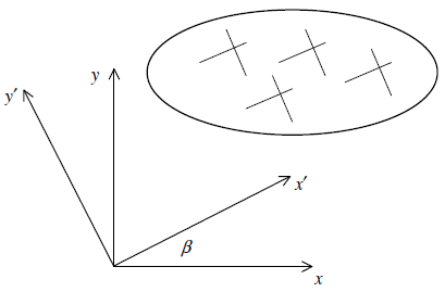
Figure 2: Shell-type element coordinate system \(xyz\) and material coordinate system \(x'y'z'\)

Determination of Orthotropic Elastic Material Properties

The material-stiffness matrices \(\big[ {\mathbf{E}_m}' \big]\) and \(\big[ {\mathbf{E}_b}' \big]\) can be expressed in terms of the nine elastic constants in Eq. (5) via

(14)\[\begin{split}\begin{split} c'_{11} &= C'_{11} - {{C'_{13} C'_{13}} \over {C'_{33}}} \\ c'_{22} &= C'_{22} - {{C'_{23} C'_{23}} \over {C'_{33}}} \\ c'_{33} &= C'_{44} \\ c'_{12} &= C'_{12} - {{C'_{13} C'_{23}} \over {C'_{33}}} \end{split}\end{split}\]

They can also be expressed in terms of the effective Poisson’s ratios \((\nu_{x'}, \nu_{y'})\), effective moduli \((E_{x'}\) and \(E_{y'})\) and shear modulus \((G)\) for orthotropic plates (Ugural [1981], p. 141):

(15)\[\begin{split}\begin{split} c'_{11} &= {{E_{x'}} \over {1 - \nu_{x'} \nu_{y'}}} \\ c'_{22} &= {{E_{y'}} \over {1 - \nu_{x'} \nu_{y'}}} \\ c'_{33} &= G \\ c'_{12} &= {{E_{x'} \nu_{y'}} \over {1 - \nu_{x'} \nu_{y'}}} = {{E_{y'} \nu_{x'}} \over {1 - \nu_{x'} \nu_{y'}}} \end{split}\end{split}\]

Ugural (1981) states that the orthotropic plate moduli and Poisson’s ratios are obtained by tension and shear tests, as in the case of isotropic materials.

When it is not possible to determine the orthotropic plate moduli and Poisson’s ratios experimentally, an equivalent or transformed orthotropic plate (with elastic properties equal to the average properties of components of the original plate) can be used, for which the orthotropic membrane elastic constants are approximated with the relations in Eq. (15), and the orthotropic bending elastic constants are approximated with the rigidities:

(16)\[\begin{split}\begin{split} {c_{11}^b}' &= {12 \over t_b^3} D_{x'} \\ {c_{22}^b}' &= {12 \over t_b^3} D_{y'} \\ {c_{33}^b}' &= {12 \over t_b^3} G_{x'y'} \\ {c_{12}^b}' &= {12 \over t_b^3} D_{x'y'} \\ \end{split}\end{split}\]

\(D_{x'}\), \(D_{y'}\), \(D_{x'y'}\) and \(G_{x'y'}\) represent the flexural rigidities and the torsional rigidity of an orthotropic plate, respectively. Rigidities for some commonly encountered cases are given in Figure 3. These cases include a reinforced concrete slab with orthogonal steel bars, a plate reinforced by equidistant stiffeners, a plate reinforced by a set of equidistant ribs, and a corrugated plate. A verification problem demonstrating how to compute the rigidities for a stiffened sheet is given here.

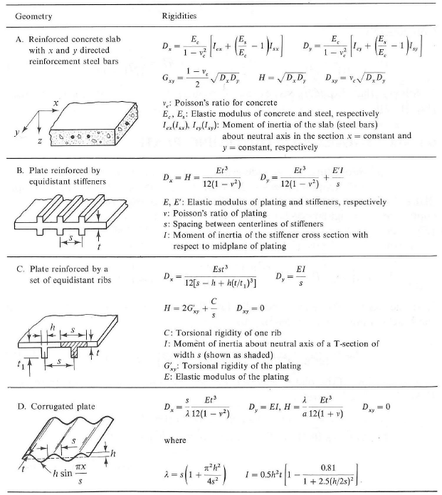
Figure 3: Rigidities of various elastic orthotropic plates (from Ugural [1981], Table 6.1)*

Note

*Used with the permission of McGraw-Hill Publishing Company.

elastic Shell Model Properties

Use the following keywords with the structure shell property (or liner/geogrid) command to set these properties of the shell isotropic elastic constitutive model.

elastic

young f

Young’s modulus, \(E\)

poisson f

Poisson’s ratio, \(\nu\)

orthotropic Shell Model Properties

Use the following keywords with the structure shell property (or liner/geogrid) command to set these properties of the shell orthotropic elastic constitutive model.

orthotropic

material-x v

material-x vector whose projection onto the shell surface defines the \(x'\)-axis of the material coordinate system. The material coordinate system, \(xʹyʹzʹ,\) satisfies the following conditions: 1) \(xʹ\) is the projection of the given vector onto the shell surface; 2) \(zʹ\) is normal to the surface and aligned with the \(z\)-axis of the element coordinate system; and 3) \(yʹ\) = \(zʹ\) × \(xʹ\). The material coordinate system moves with the shell surface during large-strain updates, which means that the relative orientations of this system and the element local system do not change (the angle \(β\) in this figure does not change). If the material-x vector is not specified, then the \(xʹ\)-axis will be aligned with the \(x\)-axis of the shell element local coordinate system. The material coordinate system can be displayed with the Shell, Geogrid and Liner plot items by choosing the System:Material attribute.

ortho-bend-constants f1 f2 f3 f4

orthotropic bending elastic constants \(\{ {c_{11}^b}', {c_{12}^b}', {c_{22}^b}', {c_{33}^b}' \}\) [F/L²] which define the bending material-stiffness matrix \(\big[ {\mathbf{E}_b}' \big]\) in the material directions \(x'y'z'\). The material directions should also be specified with the material-x property.

ortho-bend-thickness f

orthotropic bending thickness \(t_b\). If this property is not specified, then \(t_b = t\) (where \(t\) is the thickness specified via the structure shell property thickness (or liner/geogrid) command). The value of \(t_b\) should be specified after setting \(t\).

ortho-memb-constants f1 f2 f3 f4

orthotropic membrane elastic constants \(\{ {c_{11}^m}', {c_{12}^m}', {c_{22}^m}', {c_{33}^m}' \}\) [F/L²] which define the membrane material-stiffness matrix \(\big[ {\mathbf{E}_m}' \big]\) in the material directions \(x'y'z'\). The material directions should also be specified with the material-x property.

ortho-memb-thickness f

orthotropic membrane thickness \(t_m\). If this property is not specified, then \(t_m = t\) (where \(t\) is the thickness specified via the structure shell property thickness (or liner/geogrid) command). The value of \(t_m\) should be specified after setting \(t\).

anisotropic Shell Model Properties

Use the following keywords with the structure shell property (or liner/geogrid) command to set these properties of the shell anisotropic elastic constitutive model.

anisotropic

material-x v

material-x vector whose projection onto the shell surface defines the \(x'\)-axis of the material coordinate system. The material coordinate system, \(xʹyʹzʹ,\) satisfies the following conditions: 1) \(xʹ\) is the projection of the given vector onto the shell surface; 2) \(zʹ\) is normal to the surface and aligned with the \(z\)-axis of the element coordinate system; and 3) \(yʹ\) = \(zʹ\) × \(xʹ\). The material coordinate system moves with the shell surface during large-strain updates, which means that the relative orientations of this system and the element local system do not change (the angle \(β\) in this figure does not change). If the material-x vector is not specified, then the \(xʹ\)-axis will be aligned with the \(x\)-axis of the shell element local coordinate system. The material coordinate system can be displayed with the Shell, Geogrid and Liner plot items by choosing the System:Material attribute.

aniso-bend-constants f1 f2 f3 f4 f5 f6

anisotropic bending elastic constants \(\{ {c_{11}^b}', {c_{12}^b}', {c_{13}^b}', {c_{22}^b}', {c_{23}^b}', {c_{33}^b}' \}\) [F/L²] which define the bending material-stiffness matrix \(\big[ {\mathbf{E}_b}' \big]\) in the material directions \(x'y'z'\). The material directions should also be specified with the material-x property.

aniso-bend-thickness f

anisotropic bending thickness \(t_b\). If this property is not specified, then \(t_b = t\) (where \(t\) is the thickness specified via the structure shell property thickness (or liner/geogrid) command). The value of \(t_b\) should be specified after setting \(t\).

aniso-memb-constants f1 f2 f3 f4 f5 f6

anisotropic membrane elastic constants \(\{ {c_{11}^m}', {c_{12}^m}', {c_{13}^m}', {c_{22}^m}', {c_{23}^m}', {c_{33}^m}' \}\) [F/L²] which define the membrane material-stiffness matrix \(\big[ {\mathbf{E}_m}' \big]\) in the material directions \(x'y'z'\). The material directions should also be specified with the material-x property.

aniso-memb-thickness f

anisotropic membrane thickness \(t_m\). If this property is not specified, then \(t_m = t\) (where \(t\) is the thickness specified via the structure shell property thickness (or liner/geogrid) command). The value of \(t_m\) should be specified after setting \(t\).

Shell Plastic Constitutive Models

The plastic constitutive models update the internal element forces by integrating the internal stress over the shell volume using a numerical integration scheme. Stiffness matrices are not formed. There are a group of integration points distributed throughout the volume of each shell element as shown in Figure 4. The stress state satisfies the plane-stress condition such that the only non-zero components are \(\sigma_{xx}\), \(\sigma_{yy}\) and \(\sigma_{xy}\). The total stress at each integration point is updated by the shell plastic constitutive model during each timestep. There are three shell plastic constitutive models, each of which is a plane-stress version of the corresponding 3D model used by the zones. The constitutive models are von Mises, Mohr Coulomb, and Strain Softening/Hardening Mohr Coulomb. The first model is suitable for modeling steel shells, and the remaining two models are suitable for modeling concrete shells. Plasticity is provided by the DKT, CST and DKT-CST finite elements. The formulation of nonlinear structural elements that provide shell plasticity is provided in Potyondy (2022).

The integration-point layout is shown in Figure 4. The three-point triangular integration scheme with integration points at the mid points of element edges (Cowper, 1973) is used for integration over the element area. Gauss quadrature is used for integration through the thickness; the integration points are offset from the element surface, and thus, the scheme does not directly account for yielding on the surface as soon as it occurs.

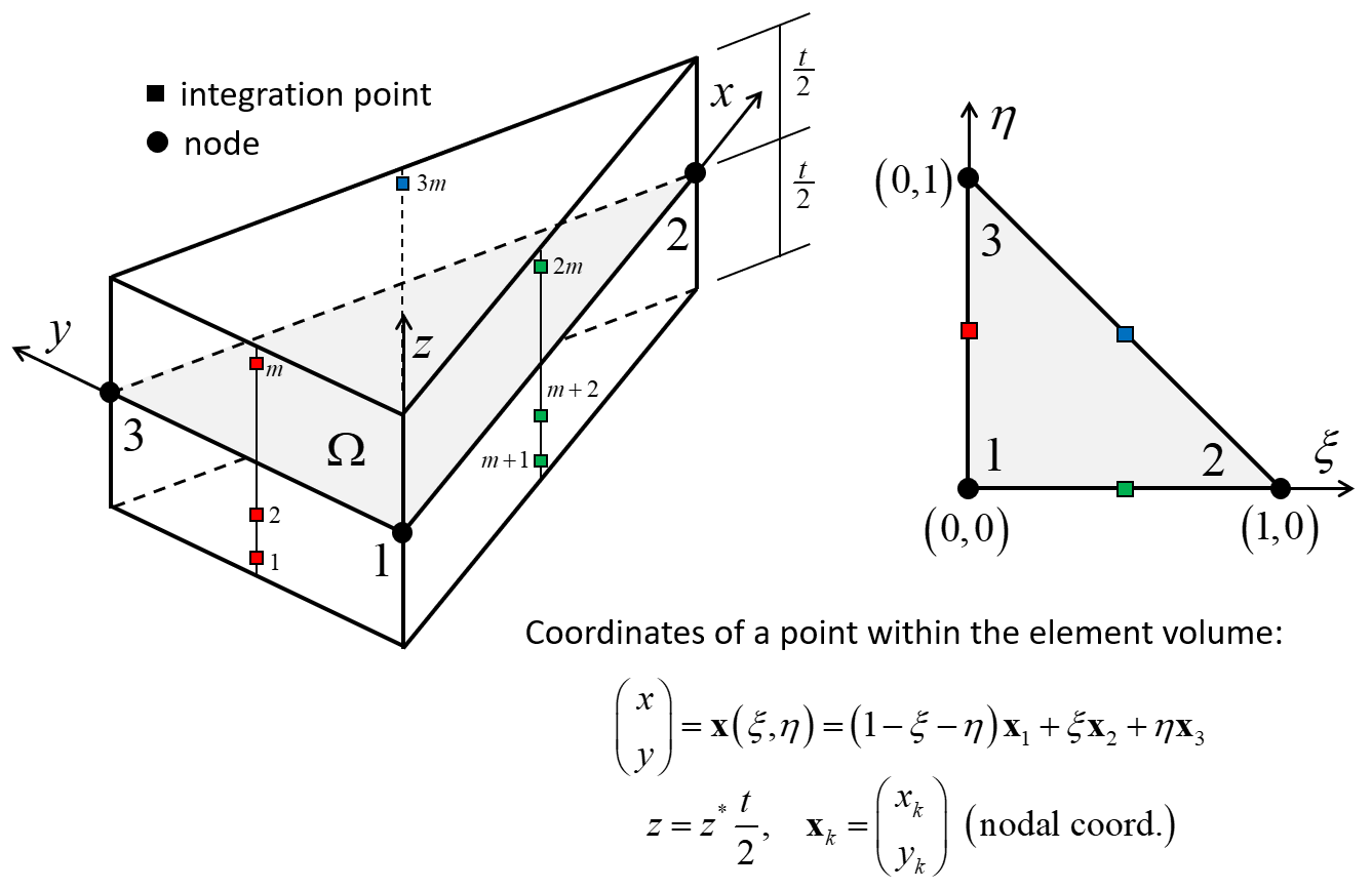
Figure 4: Triangular flat shell element with integration points throughout the shell volume for the integration scheme with three integration points over the element area. For the integration scheme with one integration point over the element area, the integration points are stacked at the element centroid with the first point near the shell bottom where \(z = -t/2\).

Burgoyne and Crisfield (1990) tested the overall performance of numerical procedures for the integration of stresses through the thickness of plates and shells when there are discontinuities in the stresses. They concluded that if integration is always required over the same range, then use Gauss quadrature, and use as high an order formula as possible, being aware that a law of diminishing return applies once nine integration points are used. This statement applies to the integration through the thickness; therefore, these integration points are to be distributed through the thickness to coincide with the Gauss abscissae for a given integration order. Their conclusion is supported by measuring the integration error for typical bending problems with yield representative of concrete and steel (see Figure 5). Guidance for choosing the number of integration points through the thickness is given in this Figure.

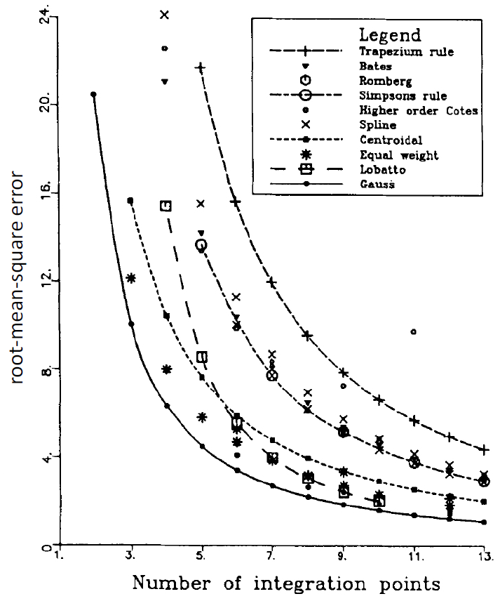
Figure 5: Comparison of numerical integration techniques demonstrating the superiority of Gauss quadrature. (From Burgoyne and Crisfield [1990])

The constitutive model (and its properties) and integration-point layout (number of integration points through the thickness and over the area) must be specified for each plastic element. The constitutive model and integration-point layout are specified with the structure shell cmodel (or liner/geogrid) command. The stresses and plastic state are listed with the plastic-stress and plastic-state keywords of the structure shell list (or liner/geogrid) command. Histories of the plastic stress are sampled with the ipstress{xx, yy, xy} keywords of the structure shell history (or liner/geogrid) command. Contours of stress, extent of yielding and yielded state are provided by the Shell, Liner and Geogrid plot items (described here).

References

Burgoyne, C. J., and M. A. Crisfield. “Numerical Integration Strategy for Plates and Shells,” Int. J. Num. Meth. Engng., 29, 105–121 (1990).

Cowper, G. R. “Gaussian Quadrature Formulas for Triangles,” Int. J. Num. Meth. Engng., 7, 405–408 (1973).

Potyondy, D. “Nonlinear Structural Elements,” Itasca Consulting Group, Inc., Technical Memorandum 5-8121:22TM36 (September 9, 2022), Minneapolis, Minnesota (2022).

Ugural, A. C. Stresses in Plates and Shells, New York: McGraw-Hill Publishing Company, Inc. (1981).

Endnotes

[1]

The shell isotropic elastic constitutive model and all of the plastic constitutive models use a single thickness \((t)\) specified via the structure shell property thickness (or liner/geogrid) command, and \(t_m = t_b = t\) in the equations of this section.

[2]

The shell orthotropic and anisotropic constitutive models use \(t_m\) and \(t_b\) to form the material-rigidity matrices and compute stresses via Eq. (3); all other thickness-related computations, such as obtaining nodal mass from element volume and density, use \(t\).