Structural Elements
An important aspect of geomechanical analysis and design is the use of structural support to stabilize a rock or soil mass. Structures of arbitrary geometry and properties, and their interaction with a rock or soil mass, can be modeled. This section describes the types of structural-support members (cables, hybrid bolts, beams, piles, shells, geogrids and liners), or structural elements, available in the program, as well as the numerical formulation that supports the structural-element logic.
The structural elements can either be independent of, or coupled to, the grid representing the solid continuum. The structural-element logic is implemented with the same explicit, Lagrangian solution procedure as the rest of the code (as opposed to an implicit, matrix-inversion procedure): the full dynamic equations of motion are solved, even for modeling processes that are essentially static. Large displacements, including geometric nonlinearity, can be accommodated by specifying a large-strain solution mode; and the full dynamic response of the system in the time domain can also be obtained with the dynamic-analysis option.
The content of this page, which provides a lengthy introduction to structural elements, is organized as follows.
We begin with a brief description of the seven types of structural-support members provided in the program.
This is followed, in Terminology, by a high-level introduction describing the relevant terminology.
The means by which structural elements are created and joined to one another is discussed next (in Geometry Creation) and Joining Structural Elements). The discussion includes a description of how particular physical entities (e.g., physical beams) that are composed of a collection of beam structural elements and nodes can be referred to — for purposes of plotting and specification of property and boundary conditions — as a single unit. The general procedures are also described for:
specification of boundary and initial conditions (in Specifying Boundary and Initial Conditions),
stresses in shells (in Stresses in Shells),
coordinate systems and sign conventions (in Local Systems and Sign Conventions),
damping conditions (in Specifying Damping and Timestep Conditions),
thermal expansion (in Thermal Expansion in Structural Elements), and
material properties (in Material Properties).
2D/3D Equivalence - Property Scaling (FLAC2D only) (in Spacing)
It is helpful to discuss the various conditions that can be prescribed at structural nodes before describing each of the types of structural elements in the program. This is done in the section on Structural Element Nodes that follows this page. This section also includes a summary of the commands associated with nodes.
In the sections the nodes section, each type of structural element is described in detail in Beam, Cable, Pile, Shell, Geogrid, and Liner Structural Elements. This includes a description of the mechanical behavior, the required properties and associated commands. Simple examples follow, illustrating the application of the given structural-element type. Finally, the reference documentation for the commands and FISH used with the particular structural element type are provided.
A detailed discussion of the general formulation of the structural-element logic is provided in General Formulation of Structural-Element Logic. Users wishing to implement more complex interaction between structural elements and the grid should consult this section to gain an understanding of the implementation procedure.
Throughout this section, matrices and vectors will be denoted by boldface type. The mathematical symbols \([\quad ]\), \(\lceil\quad\rfloor\), \(\{\quad\}\) and \(\lfloor\quad\rfloor\) will designate a rectangular matrix, diagonal matrix, column vector and row vector, respectively. Also, structure and element matrices will be described by uppercase and lowercase English alphabet characters. For example, \([\bf K]\) and \([\bf k]\) designate structure and element stiffness matrices, respectively.
Types of Structural Elements
Seven types of structural-support members can be specified. Each of these members can be joined to one another and/or the grid.
Cable Structural Elements — Cable structural elements are two-noded, straight, finite elements with one axially oriented translational degree-of-freedom per node. A physical cable (i.e., an arbitrarily curved, cable structure of isotropic material) can be modeled as a collection of cable elements. Each element can yield in tension or compression, but cannot resist a bending moment. A shear-directed (parallel with the cable axis) frictional interaction occurs between the cable and the grid. A cable may be anchored at a specific point in the grid, or grouted so that force develops along its length in response to relative motion between the cable and the grid. Cables may also be point-loaded or pretensioned. Cable elements are used to model a wide variety of structural-support members for which tensile capacity is important, including cable bolts and tiebacks.
Hybrid-Bolt Structural Elements — Hybrid-bolt structural elements are cables with a spring added wherever the cable crosses an interface or joint. The spring, or “dowel” acts to resist shearing on the joint.
Beam Structural Elements — Beam structural elements are two-noded, straight, finite elements with six degrees of freedom per node: three translational components, and three rotational components. A physical beam (i.e., an arbitrarily curved, beam structure of isotropic material and bisymmetrical cross-section) can be modeled as a collection of beam elements. The beam elements behave either as an isotropic, linearly elastic material with no failure limit or as a plastic material. There is one elastic, and three plastic constitutive models. When using the elastic constitutive model, the beam may be either an Euler-Bernoulli beam that is appropriate for modeling long thin beams, or a Timoshenko beam that is appropriate for modeling short thick beams. One can introduce a limiting plastic moment, or even a plastic hinge (across which a discontinuity in rotation may develop), between elements. Beam elements may be rigidly connected to the grid such that forces and bending moments develop within the beam as the grid deforms, and they may be loaded by point or distributed loads. Beam elements are used to model structural-support members in which bending resistance and limited bending moments occur, including support struts in an open-cut excavation and general framed structures loaded by point or distributed loads.
Pile Structural Elements — Pile structural elements are two-noded, straight, finite elements with six degrees of freedom per node. A physical pile can be modeled as a collection of pile elements. The stiffness matrices and plastic constitutive models of a pile element are identical to those of a beam element; however, in addition to providing the structural behavior of a beam, both a normal-directed (perpendicular to the pile axis) and a shear-directed (parallel with the pile axis) frictional interaction occurs between the pile and the grid. In this sense, piles offer the combined features of beams and cables. In addition to skin-friction effects, end-bearing effects can also be modeled (see Axially Loaded Pile). Piles may be loaded by point or distributed loads. Pile elements are used to model structural-support members, such as foundation piles, for which both normal- and shear-directed frictional interaction with the rock or soil mass occurs.
A special material model is also available as an extension to the pile element to simulate the behavior of rockbolt reinforcement. This model includes the ability to account for changes in confining stress around the reinforcement, strain-softening behavior of the material between the structural element and the grid, and tensile rupture of the element.
Shell Structural Elements — Shell structural elements are three-noded, flat finite elements. Five finite-element types (2 membrane elements, 1 plate-bending element and 2 shell elements) are available. A physical shell (i.e., an arbitrarily curved, shell structure of either isotropic or orthotropic material) can be modeled as a faceted surface composed of a collection of shell elements. The structural response of the shell is controlled by the finite-element type (to resist membrane loading only, bending loading only, or both membrane and bending loading). The shell elements behave either as an isotropic or orthotropic, linearly elastic material with no failure limit or as a plastic material. There are three elastic, and three plastic constitutive models. One can introduce a plastic-hinge line (across which a discontinuity in rotation may develop) along the edges between elements, using the same double-node procedure as is applied to beams. Shell elements may be rigidly connected to the grid such that stresses develop within the shell as the grid deforms, and they may be loaded by point loads or surface pressures. Shell elements are used to model the structural support provided by any thin-shell structure in which the displacements caused by transverse-shearing deformations can be neglected.
Geogrid Structural Elements — Geogrid structural elements are three-noded, flat, finite elements that are assigned a finite-element type that resists membrane but does not resist bending loading. A physical membrane can be modeled as a collection of geogrid elements. The geogrid elements behave either as an isotropic or orthotropic, linearly elastic material with no failure limit or as a plastic material. A shear-directed (in the tangent plane to the geogrid surface) frictional interaction occurs between the geogrid and the model grid, and the geogrid is slaved to the grid motion in the normal direction. A geogrid can be anchored at a specific point in the model grid, or attached so that stress develops along its surface in response to relative motion between the geogrid and the model grid. The geogrid can be thought of as the two-dimensional analog of a one-dimensional cable. Geogrid elements are used to model flexible membranes for which shear interaction with the soil is important, such as geotextiles and geogrids.
Liner Structural Elements — Liner structural elements are three-noded, flat finite elements that can be assigned any of the five finite-element types available for shell elements. A physical liner can be modeled as a collection of liner elements that are attached to the surface of the model grid. The liner elements behave either as an isotropic or orthotropic, linearly elastic material with no failure limit or as a plastic material. In addition to providing the structural behavior of a shell, a shear-directed (in the tangent plane to the liner surface) frictional interaction occurs between the liner and the model grid. Also, in the normal direction, both compressive and tensile forces can be carried, and the liner may break free from (and subsequently come back into contact with) the grid. Liner elements are used to model thin liners for which both normal-directed compressive/tensile interaction and shear-directed frictional interaction with the host medium occurs, such as shotcrete-lined tunnels or retaining walls.
The liner may also be embedded within the grid such that it interacts with the grid on both sides of the liner.
Terminology
The structural-element logic allows one to model the structural response of a mechanical system that is composed of a solid continuum and a framework of load-carrying members. The solid continuum is represented by a collection of polyhedral-shaped zones, each of which is associated with a set of gridpoints. The framework is represented by a collection of structural elements, each of which is associated with a set of nodes. The framework interacts with the solid continuum by means of links which connect nodes to zones (not simply to gridpoints) or to other nodes.
Six degrees of freedom, composed of three translational components and three rotational components, are associated with each node. Each node also has its own local orthogonal coordinate system. The node-local system provides the directions in which the equations of motion for the node are solved, and also defines the directions in which the node can be attached to a target entity via a link. A link supports the following three attachment conditions, which are specified independently for each local direction of its source node: free, rigid and deformable. See Structural-Element Links for a detailed description of structural-element links.
For most modeling situations, it is not necessary to specify link properties; instead, it is sufficient to create, position and assign properties to the desired structural elements. Nodes (and links, if necessary) will be created automatically, and will inherit necessary information from the structural elements that use them.
Geometry Creation
The seven types of structural elements provide the building blocks, or components, needed to model seven types of physical items: cables, hybrid-bolts, beams, piles, shells, geogrids and liners. Each physical item is associated directly with a collection of component objects of the same type. For example, a cable is associated with a collection of cable elements, whereas a liner is associated with a collection of liner elements. The association between physical items and their corresponding component objects is implemented by storing two distinct identification numbers for each structural element:
id— The ID number refers to the physical item.component-id— The component-ID number refers to the component object itself.
Properties may be specified for each type of physical item, and will be inherited automatically by the associated component objects. For example, the command
struct cable property grout-friction=30.0 range id=3
will assign a grout friction angle of 30 degrees to all cable elements that are part of the cable with an ID number of 3, whereas the command
struct cable property grout-friction=30.0 range component-id=3
will assign a grout friction angle of 30 degrees to the single cable element with a component-ID number of 3.
The Cable, Hybrid-Bolt (and Dowel), Beam, Pile, Shell, Geogrid, and Liner plot items allow one to view the seven different element types, as well as the nodes and the links.
Cable, Hybrid-Bolt, Beam and Pile Structural Elements
The geometry of cables, hybrid bolts, beams and piles is defined by their corresponding collection of component objects. The creation commands for all four of these types are identical, and for simplicity the following examples will be for cable elements, but they will work just as well for hybrid, pile or beam elements.
A single cable forming a straight line (made up of a number of individual elements) can be created using the structure cable create command, in one of three ways:
By specifying the two end locations (
structure cable create by-line),By specifying the ID numbers of two nodes at each end (
structure cable create by-nodeids), orBy specifying a starting point, a direction, and a length (
structure cable create by-ray).
Each create command takes an optional ID argument to denote the ID of the item to be created. If no ID is provided, the next available ID will be used. New nodes are created automatically at uniformly spaced internal points along the line. If a node already exists at one of the end locations and is used by a element with the same ID as that given in the command, a new node is not created at this location; otherwise, a new node is created.
A group of cables may be created from external geometric information, using the structure cable import command. For each line segment in the imported data, one or more cable elements will be created. Currently, data can be imported in one of three ways:
From an existing geometry set (
structure cable import from-geometry). See the Geometry for details of creating a geometric set.From a compatible CAD file (
structure cable import from-file). The currently compatible file types are DXF, STL, and the Itasca Geometry format.From a Sketch set (
structure cable import from-sketch). See the Sketch for how to create geometry in Sketch.
The following example, depicted in Figure 1, illustrates the association mechanism between nodes and structural elements. The nodes are not drawn in these plots. Instead, the cable elements are drawn at 90% of their true length. Consider a curved cable, identified by an id of 5, that is composed of a collection of 7 elements and 8 nodes. Each element stores the cable id of 5, as well as its own unique component-id. This can be seen by moving the mouse over an element and examining the information window. In this way, the 7 elements are combined to form a complex, arbitrarily curved cable that can be referred to by the single id of 5.
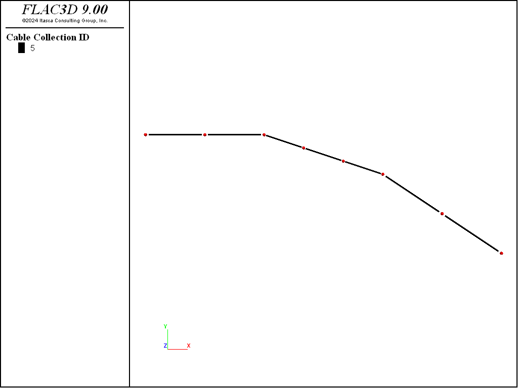
Figure 1: Representation of a single curved cable identified by an ID of 5
The commands necessary to produce the model are shown in Figure 1 are given in selexample1-1.dat.
selexample1-1.dat: Creating a single curved cable identified by an ID of 5
model new
structure cable create by-line (0.0,4.0,0.0) (3.0,4.0,0.0) segments=2 id=5
structure cable create by-line (3.0,4.0,0.0) (6.0,3.0,0.0) segments=3 id=5
structure cable create by-line (6.0,3.0,0.0) (9.0,1.0,0.0) segments=2 id=5
There is no restriction that requires the end locations to lie within the model grid; in fact, it is not necessary to have a grid at all. (Recall that the structural elements can either be independent of, or coupled to, the grid representing the solid continuum.) When using the structure cable create command, if any of the nodes used by the newly created elements lie within zones, these nodes will be linked to these zones, and the link properties will be set consistent with the corresponding element behavior described in Cable, Hybrid Bolt, Beam and Pile Structural Elements.
The most common reason to specify more than one segment between end locations is to improve accuracy, especially with piles and cables that are interacting with the host medium. In this case, the distribution of shear forces along each pile or cable is a function, to some extent, of the number of nodes. The following rules-of-thumb have been used to determine the number of nodes to use when modeling cables:
Try to provide approximately one node in each zone. The reasoning here is that since the zones are constant-stress regions, it is not necessary to have more than one interaction point within a zone.
Try to provide two to three cable element within the development length of the cable. The development length of the cable is determined by dividing the specified yield strength, \(F_t\), by the grout cohesive strength, \(c_g\). By following this procedure, failure by “pull-out” can occur if such conditions arise. If the cable elements are too long, then only the yield failure mode of each element is possible. (This reasoning also applies to pile elements if used to simulate the behavior of rockbolts.)
Shell, Geogrid and Liner Structural Elements
The geometry of shells, geogrids and liners is defined by their corresponding collection of component objects. The creation commands for all three of these types are identical, and for simplicity the following examples will be for shell elements, but they will work just as well for geogrid or liner elements.
A single shell surface (made up of a number of individual elements) can be created using the structure shell create command, in one of five ways:
By specifying a set of surface FLAC3D zone faces, on which elements will be created (
structure shell create by-zone-face).By specifying a set of surface 3DEC zone faces, on which elements will be created (
structure shell create by-block-face).By specifying four existing structural nodes, forming a quadrilateral (
structure shell create by-nodeids).By specifying four points in space, forming a quadrilateral (
structure shell create by-quadrilateral).By specifying three points in space, forming a triangle (
structure shell create by-triangle).
A shell surface may also be created from external geometric information, using the structure shell import command. For each line segment in the imported data, one or more shell elements will be created. Current, data can be imported in one of two ways:
From an existing geometry set (
structure shell import from-geometry). See the Geometry for details of creating a geometric set.From a compatible CAD file (
structure shell import from-file). The currently compatible file types are DXF, STL, and the Itasca Geometry format.
The most common way that shell-type elements are created in the program is with the structure shell create by-zone-face command, which places them on zone faces. As an example below, the geometry logic is used to create a 45 degree arc surface of shell elements. The command used as listed in selexample1-2.dat.
The geometry edge create by-arc command is used to create a 45 arc section in 8 segments. Then the geometry generate from-edges command is used to extrude those edges in the \(y\)-direction into 8 segments. This description is then used by the structure shell import from-geometry command to create two triangular shell elements per quadrilateral in the geometric description. Figure 2 shows the resulting shell elements.
model new
geometry select 'cyl'
geometry edge create by-arc origin (0,0,0) start (0,0,1)...
                            end (0.707,0,0.707) segments 8
geometry generate from-edges extrude (0,1,0) segments 8
structure shell import from-geometry 'cyl'
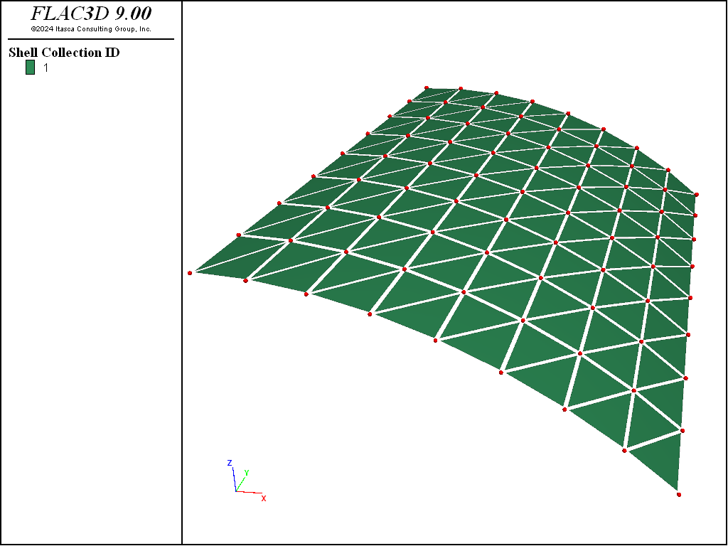
Figure 2: Representation of a curved shell created by generating shell elements using a geometry description
Joining Structural Elements to One Another and to the Grid
Structural elements can be joined to one another either by sharing a node or by having one of their nodes linked to either another node or to a zone (see Terminology). If two or more structural elements share a node, all forces and moments are transferred between the elements at the node. If it is necessary to limit or eliminate specific forces and/or moments that are transferred between elements, then two separate nodes may be created and connected by a node-to-node link, and the appropriate attachment conditions set. For example, if it is necessary to join two beams with a ball-joint, a node-to-node link can be added between the two beam end nodes, and the attachment conditions set in all translational and rotational directions to be rigid and free, respectively. The same procedure can be applied when joining elements to the grid, except that in this case, a node-to-zone link must be established between the node and the zone in which it lies. Node-to-node and node-to-zone linkage is controlled via the structure link command, and the linkage conditions are described in Structural-Element Links.
The element creation commands ( structure cable create, structure beam create, etc.) are designed to maintain a clear separation between different physical items being modeled. For example, if modeling two separate piles lying end-to-end, issue two separate structure pile create commands and specify two separate IDs (e.g., 1 and 2). This will result in the creation of two nodes lying in the same geometric location: one is used by pile-1; one is used by pile-2. Forces and moments will not be transferred between the adjoining pile elements; instead, only forces will be transmitted into the surrounding zone at the common location. This mimics two separate piles lying end-to-end. If a single pile is desired, then issue two separate structure pile create commands, but this time specify the same ID for each. This will result in the creation of a single node that is shared by the pile element on each side of the common location. Forces and moments will be transferred between the adjoining elements. In most modeling situations, the default link attachment conditions that are set by the element creation commands should not be modified, because these attachment conditions produce the desired element-grid interaction for each particular element type.
Specifying Boundary and Initial Conditions
All boundary and initial conditions (with the exception of distributed loads applied to beam and pile surfaces, pressure loads applied to shell, liner, and geogrid surfaces, and pretension forces applied to cables) are specified with the structure node command. The nodal conditions include
velocity-fixity conditions,
current velocity components, and
applied point loads (forces and/or moments).
There are two coordinate systems associated with each node: the global system and the node-local system. The node-local system is used to specify attachment conditions that control how the node interacts with the grid. Also, the equations of motion are solved in these local directions. Therefore, one may fix or free velocities in these directions only. The orientation of the node-local system is set automatically at the start of a set of cycles based on the type of elements that use the node. (See the structure node command for a full description of these two systems.)
Velocities and rotations at nodes are fixed and freed in the node-local system using the structure node fix and structure node free commands. Velocities and rotations are initialized to specified values in the global system using the structure node initialize command. Point loads are applied at nodes in either the global or the node-local system using the structure node apply command.
Distributed loads are applied to elements using the structure cable apply (for example). Linear elements (beam, cable, or pile) can apply distributed loads in the element local y and z directions. Planar elements (shell, geogrid, or liner) can apply pressure normal to the element surface. Note that in large-strain mode, the applied loads remain aligned with the corresponding element system directions, which may rotate as the element location changes.
Pretension forces are applied to cables using the structure cable apply tension command. A positive pretension force places the cable into tension. See Pretensioning for additional information.
Stresses in Shells
This section provides a brief introduction to shell behavior. Much of the information in this section is taken from Cook et al. (1989, 2002). Consult those texts for a more complete discussion.
A shell forms a curved surface in space. Usually a shell is thin in comparison with its span. Geometrically, a shell is described by its thickness, \(t\), and the shape of the shell mid-surface. If the mid-surface is flat, then the shell is called a plate. In general, a shell simultaneously displays bending stresses and membrane stresses. Bending stresses in a shell correspond to bending stresses in a plate and produce bending and twisting moments and transverse-shear forces. Membrane stresses correspond to stresses in a plane-stress problem: they act tangent to the mid-surface, and produce mid-surface tangent forces. These moments and forces per unit length are called stress resultants. There are a total of eight stress resultants, which can be divided into those that arise from bending action and those that arise from membrane action. These will be described in the following two sections.
Bending Action
We can account for the bending action of a shell in terms of plate-bending theory, which extends beam theory from one dimension to two as follows. Define a surface coordinate system \(xyz\) such that \(x\) and \(y\) are orthogonal coordinates in the mid-surface and \(z\) is a direction normal to the mid-surface. Approximate the tangent plane to the shell mid-surface as a flat plate subjected to “plate bending,” meaning that external loads have no components parallel to the \(xy\)-plane and that \(\sigma_{xx}\) = \(\sigma_{yy}\) = \(\sigma_{xy}\) = 0 on the mid-surface \(z=0\). Such a flat plate, like a straight beam, supports transverse loads by bending action. Figure 3 shows stresses that act on cross sections of a plate whose material is homogeneous and linearly elastic, subjected to plate-bending loading. Normal stresses \(\sigma_{xx}\) and \(\sigma_{yy}\) vary linearly with \(z\), and are associated with bending moments \(M_x\) and \(M_y\). Shear stress \(\sigma_{xy}\) also varies linearly with \(z\), and is associated with twisting moment \(M_{xy}\). Normal stress \(\sigma_{zz}\) is considered negligible in comparison with \(\sigma_{xx}\), \(\sigma_{yy}\) and \(\sigma_{xy}\). Transverse shear stresses \(\sigma_{yz}\) and \(\sigma_{xz}\) vary quadratically with \(z\). Lateral load \(q\) includes surface load and body force, both in the \(z\)-direction.
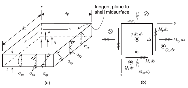
Figure 3: Bending action in a shell showing: (a) stresses that act on a differential element of a homogeneous, linearly elastic plate subjected to plate-bending loading; and (b) stress resultants corresponding with these stresses. (Stress resultants are drawn acting in their positive sense.)
Stresses in Figure 3 produce the bending stress resultants
and the transverse-shear stress resultants
The bending resultants are moments per unit length, and the transverse-shear resultants are forces per unit length. Differential total moments and forces are \(M_x\)\(dy\), \(Q_x\)\(dy\), and so on, as shown in Figure 3. The following stress distributions are consistent with the assumptions of plate-bending theory, and satisfy (1) and (2):
Stresses \(\sigma_{xx}\), \(\sigma_{yy}\) and \(\sigma_{xy}\) are largest at the surface \(z = \pm t/2\), whereas transverse-shear stresses, \(\sigma_{xz}\) and \(\sigma_{yz}\), are largest at the mid-surface. Two points should be noted:
The differential equations of equilibrium for a plate element under a general state of stress indicate that \(\sigma_{zz}\) varies as a cubic parabola over the thickness of the plate (Ugural 1981). But this stress, according to the assumptions of plate-bending theory, is negligible compared with the other stress components — this assumption becomes unreliable in the vicinity of highly concentrated transverse loads.
\(\sigma_{xz}\) and \(\sigma_{yz}\), according to the assumptions of plate-bending theory, are negligible compared with the other stress components; however, when these stresses are integrated through the thickness, they produce transverse-shear stress resultants, \(Q_x\) and \(Q_y\), that are of the same order of magnitude as the surface loading and moments.
Membrane Action
We can account for the membrane action of a shell in terms of plane-stress conditions. Define a surface coordinate system \(xyz\) such that \(x\) and \(y\) are orthogonal coordinates in the mid-surface, and \(z\) is a direction normal to the mid-surface. Approximate the tangent plane to the shell mid-surface as a flat plate subjected to plane-stress conditions, meaning that the plate is loaded in its own plane. Such a flat plate supports these loads by membrane action. Figure 4 shows stresses that act on cross sections of a plate whose material is homogeneous and linearly elastic, subjected to plane-stress loading. Normal and shear stresses \(\sigma_{xx}\), \(\sigma_{yy}\) and \(\sigma_{xy}\) are constant through the thickness.
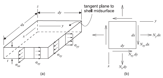
Figure 4: Membrane action in a shell showing: (a) stresses that act on a differential element of a homogeneous, linearly elastic plate subjected to plane-stress loading; and (b) stress resultants corresponding with these stresses. (Stress resultants are drawn acting in their positive sense.)
Stresses in Figure 4 produce the membrane stress resultants
The membrane resultants are forces per unit length. Differential total forces are \(N_x\)\(dy\), \(N_y\)\(dx\) and so on, as shown in Figure 4. The following stress distributions are consistent with the plane-stress assumptions and satisfy (4):
General Shell Stresses
A shell structure simultaneously displays bending stresses and membrane stresses. The stresses and stress resultants acting in a general shell consist of a superposition of these two loading modes (see Bending Action and Membrane Action). We can express these stress quantities in terms of a surface coordinate system \(xyz\), where \(x\) and \(y\) are orthogonal coordinates in the shell mid-surface and \(z\) is a direction normal to the mid-surface. The eight stress resultants can be divided into bending (\(M_x\), \(M_y\), and \(M_{xy}\)), transverse-shear (\(Q_x\) and \(Q_y\)) and membrane (\(N_x\), \(N_y\) and \(N_{xy}\)) stress resultants (see (1), (2), and (4)). The distribution of stress through the shell thickness follows from the particular plate or shell theory used to model structural behavior. For both the Kirchhoff (thin-shell) and Reissner (thick-shell) theories, the stress distributions correspond with a superposition of (3) and (5):
The stresses and stress resultants are sketched in Figure 3 and Figure 4, which also provide the sign convention for the stress resultants.
Stress Recovery Procedure
General shell stresses are computed in the program for elastic material as follows. Refer to Stress Recovery Procedure (in detail) for a more detailed description of the stress-recovery procedure, and to the structure shell recover (or liner/geogrid) command for a discussion that encompasses plastic elements. Each shell-type structural element (shell, geogrid, and liner) with an elastic material model has an associated finite-element stiffness matrix that defines the structural response (see Finite Elements). Each shell-type element stores an internal force vector containing the generalized nodal forces acting on the element. During each timestep, the internal force vector is updated by multiplying the element stiffness matrix with the incremental nodal displacements (nodal velocities multiplied by timestep). Note that shell stresses are not computed during each timestep. Shell stresses are only computed by invoking a stress-recovery procedure that uses the internal force vector and the stiffness matrix to first compute stress resultants, and then compute stresses using (6). These stress resultants are in equilibrium with the generalized nodal forces acting on the element.
The structural properties of shell-type elements with an elastic material model include material properties (e.g., \(E\) and \(\nu\) for an isotropic material) and thickness. These properties are embodied in the element stiffness matrix. If a structural property is modified during a simulation, then: (1) the generalized nodal forces and the stress resultants will remain the same; and (2) the stresses will change only if the thickness is altered (see (6) and note that a change in thickness will affect the stresses even if the stress resultants do not change).
Note that the same procedure is used for all shell-type structural elements, shell, geogrid, and liner. The command and FISH examples below use shell, but any of the shell-type keywords can be substituted.
The stress-recovery procedure requires that a consistent surface coordinate system be established prior to recovering any stress quantities. The surface coordinate system, \(xyz\), establishes \(x\) and \(y\) as orthogonal coordinates in the shell mid-surface, and \(z\) as normal to the mid-surface. The stress resultants are expressed in terms of this system. The surface coordinate system is stored at each node, and can be set with the structure shell recover surface command and the FISH function struct.node.system.surface. It can be printed with the structure node list system-surface command and plotted with the Shell, Geogrid, and Liner plot items.
After establishing the surface coordinate system over a patch of shell-type elements, stress resultants and stresses can be recovered for these elements with the structure shell recover resultants and structure shell recover stress commands. These values can be queried, sampled as histories, and viewed as colored contours:
The values can be queried with the
structure shell list resultants,structure shell list stress, andstructure shell list stress-principalcommands, and the FISH functionsstruct.shell.resultant,struct.shell.stress, andstruct.shell.stress.prin.The values can be sampled as histories with the
structure shell historycommand.The values can be plotted as color contours with the Shell, Geogrid, or Liner plot item. Note that by default the plot items calculate an up-to-date value of the resultants and stresses, but they can be set to show the current engine values in the plot item attributes.
The stress resultants and stresses become invalid after any step is taken, or if the surface coordinate system is altered; also, the stresses become invalid if the depth factor is altered. In these cases, the values must be recovered again.
The stress-recovery procedure involves two steps: (1) creation of a consistent surface coordinate system; and (2) recovery of stress quantities. Both of these steps can be limited to only apply to a range of shell-type elements. This allows one to control whether nodal averaging will occur between shell-type elements that use the same node. For example, suppose that one wished to recover stresses throughout a capped cylindrical pressure vessel. The curvature across the cap edge is not continuous, and some of the stresses across this edge are also not continuous. We could recover stresses separately in the cap and in the cylinder walls by performing two separate recovery operations for the shell-type elements in these regions. When doing so, the \(z\)-direction of the surface coordinate system for the nodes along the edge would be different in each case.
Local Systems and Sign Conventions
Each element has its own local coordinate system. For beams and piles, this system is used to specify both the cross-sectional moments of inertia and applied distributed loading. For shells, geogrids and liners, this system is used to specify orthotropic material properties and applied pressure loading.
Each node has its own node-local coordinate system. This system is used to specify attachment conditions that control how the node interacts with the grid, and also defines the directions in which the equations of motion are solved. The orientation of the node-local system is set automatically at the start of a set of cycles based on the type of elements that use the node (see the structure node command).
Responses are computed for nodes and for each type of element. Nodal responses include forces and moments, as well as translational and rotational velocities and displacements. Forces and translational velocities are positive in the direction of the positive coordinate axes (either global or node-local) at the node. Positive moments and rotational velocities follow the “right-hand rule”: With the thumb pointing in the direction of the positive coordinate axis, the fingers are curled in the positive direction of rotation. The double arrows in Figure 3 indicate the direction of the right-hand thumb to define the positive moment and rotation.
Responses for each type of element, and the associated sign conventions, are described in the sections named “Response Quantities” associated with each element type. The sign convention for force and moment distributions in beams and piles is shown in Force-Moment Sign Convention, and the sign convention for stress resultants in shells, geogrids and liners is shown in Bending Action and Membrane Action, where the \(xyz\)-axes correspond with the surface coordinate system used during stress recovery (see Stress Recovery Procedure).
Specifying Damping and Timestep Conditions
The same damping conditions applied to the model grid for static and dynamic analysis can also be applied to the structural elements. The damping conditions specified with the zone mechanical damping and zone dynamic damping commands apply only to the zones, while the structure mechanical damping and structure dynamic damping commands apply to the structural elements. The structure mechanical damping and structure dynamic damping commands can be used to change the damping type for the nodes. The timestep used for either static or dynamic analysis can be adjusted by using the structure safety-factor command. Also, the computation of the rotational degree-of-freedom masses during dynamic analysis can be controlled by the structure scale-rotational-mass command.
Thermal Expansion in Structural Elements
The effect of thermal expansion can be accounted for in the structural elements as follows. The model must be configured for thermal analysis via the model configure thermal command. Temperature increments occur at structure nodes either directly set by the struct.node.temp.increment function, or obtained from the temperature increments in the zones that are connected by links to the nodes. The effect of heat conduction in the structural element is not considered. It is assumed that the zone temperature is communicated instantaneously to the structural elements. The temperature change generates thermal expansion/contraction in the axial direction of 1D structural elements (cable, hybrid bolt, beam or pile) and in the plane of 2D structural elements (shell, geogrid or liner). The effect of the lateral expansion in the element is neglected, and no other coupling takes place.
The structural-element nodal temperature increment is determined by interpolation of nodal temperature increments in the host zone. For a 1D structural element, the temperature change is calculated as the average of values at the two nodes. The thermal strain increment of a 1D element is computed as the product of the thermal-expansion coefficient, temperature change for the step, and element length. For a 2D structural element, the temperature change is calculated as the average of values at the three nodes. The thermal strain increment of a 2D element is computed as the product of the thermal-expansion coefficient, temperature change for the step, and the lengths of the vectors from the element centroid to each node. (There are three of these vectors.) Thermal strains, thermal strain increments and temperatures at structural nodes are not stored.
Note that when a large temperature increment is specified for cables, it is advisable to assign nonzero compressive yield strength to the cables in order to avoid compressive yielding during the thermal expansion stage.
Material Properties
Properties are assigned to structural elements with the structure shell property command (or the equivalent for beam, cable, pile, geogrid, or liner elements). The range logic can be used to limit the property settings to only those elements within the specified range. The properties for each structural-element type are described in detail in the following sections. Note that all quantities must be given in a consistent set of units (see Table 1).
Property |
Unit |
SI |
Imperial |
||||
|---|---|---|---|---|---|---|---|
area |
length2 |
m2 |
m2 |
m2 |
cm2 |
ft2 |
in2 |
axial or shear stiffness |
force/disp |
N/m |
kN/m |
MN/m |
Mdynes/cm |
lbf/ft |
lbf/in |
exposed perimeter |
length |
m |
m |
m |
cm |
ft |
in |
moment of inertia |
length4 |
m4 |
m4 |
m4 |
cm4 |
ft4 |
in4 |
plastic moment |
force-length |
N-m |
kN-m |
MN-m |
Mdynes-cm |
ft-lbf |
in-lbf |
yield strength |
force |
N |
kN |
MN |
Mdynes |
lbf |
lbf |
Young’s modulus |
stress |
Pa |
kPa |
MPa |
bar |
lbf/ft2 |
psi |
where, 1 bar = 106 dynes/cm2 = 105 N/m2 = 105 Pa.
Structural Elements in FLAC2D
The following content is specific to structural elements in FLAC2D only. Topics include:
Plane-stress vs. Plane-strain Structural Elements
Beam, cable, pile and rockbolt elements adhere to a plane-stress formulation. If the element is representing a structure that is continous in the direction perpendicular to the analysis plane (e.g. a concrete tunnel lining), the value of \(E\) must be divided by \((1 - \nu^2)\) to account for plane-strain conditions. Note that beam, cable, pile and rockbolt elements cannot be used to simulate a single vertical element because the structural element forumlation does not currently support axisymmetry conditions. For such a case, FLAC3D is recommended.
Liner elements in FLAC2D are typically assumed to be continous in the direction perpendicular to the analysis plane, therefore the Young’s modulus (\(E\)) is automatically divided by \((1 - \nu^2)\) to account for plane-strain conditions. Additionally, since liner elements behave as continous plain-strain elements, spacing is not an option. More information regarding liners in FLAC2D can be found in the Liner Structural Elements (2D) section.
2D/3D Equivalence - Property Scaling (Spacing)
Reducing 3D problems (with regularly spaced beams, cable, piles or rockbolts) to 2D problems involves averaging the effect in 3D over the distance between the elements. Donovan et al. (1984) suggests that the linear scaling of material properties is a simple and convenient way of distributing the discrete effect to elements over the distance between elements in a regularly spaced pattern.
The relation between actual properties and scaled properties can be demonstrated by considering the coupling strength properties for regularly spaced piles. The actual maximum coupling normal force for pile element is defined as
where (\(F_n^{max}\)) is the maximum normal force per unit model thickness, \(c_n\) is the coupling normal cohesion, \(\sigma_n\) is the effective confining stress (given here (2)), \(\phi_n\) is the coupling normal friction angle and \(p\) is the perimeter. Internally, FLAC2D uses the scaled expression
where (\({\bf F_n^{max}}\)) is the scaled maximum normal force per unit model thickness calculated by FLAC2D (bold lettering indicates scaled values). We want the total force calculated by FLAC2D over a spacing, \(S\), to be the same as the actual force. The actual maximum coupling normal force is then
and the actual coupling normal force is
The relation between the actual force and the FLAC2D force can be satisfied by substituting (9) and the following relations into (8).
The actual normal stress on the pile, \(\sigma_n\), is calculated by dividing teh actual force by the acutal effective area (perimeter \(\times\) length, \(pL\)):
Note that the choice to scale friction is arbitrary, because only the product \(tan(\phi_n) \times p\) is relevant. Alternatively, the perimeter term could be scaled.
It is important to remember that the forces (and the moments) for structural elements that are calculated by FLAC2D are scaled forces (and moments). If spacing is not specified the actual forces and moments can be calculated by multiplying the FLAC2D force and moments by \(S\). FISH, plotting and histories will access scaled values of forces and moments, and thus these values should be multiplied by the appropriate spacing to determine the actual values.
The spacing property is provided with beams, cables, piles and rockbolts to scale the properties, and account for a spaced pattern of these structural elements. When spacing is specified in the structure beam property (or cable, pile)
command, the actual properties of the structural elements are input. The scaled properties are then calculated automatically by dividing the actual properties by the spacing, \(S\). When the calculation is complete, the actual force and moments
in the spaced structural elements are then determined automatically (by multiplying by the spacing, \(S\)) which are accessible in FISH, histories and plotting.
The following lists summarize the structural element properties that are scaled when the spacing property is specified to simulate regularly spaced structural elements.
Property |
Beams |
Cables |
Piles |
Rockbolts |
|---|---|---|---|---|
\(E\) (Young’s modulus) |
\(E\) |
\(E\) |
\(E\) |
\(E\) |
\(M^P\) (plastic moment) |
\(M^P\) |
\(M^P\) |
\(M^P\) |
|
\(V^P\) (plastic shear) |
\(V^P\) |
\(V^P\) |
\(V^P\) |
|
\(F_t\) (tensile yield strength) |
\(F_t\) |
\(F_t\) |
||
\(F_c\) (compressive yield strength) |
\(F_c\) |
\(F_c\) |
||
\(k_g\) (grout stiffness) |
\(k_g\) |
|||
\(\phi_g\) (grout friction) |
\(\phi_g\) |
|||
\(k_s\) (coupling shear stiffness) |
\(k_s\) |
\(k_s\) |
||
\(c_s\) (coupling shear cohesion) |
\(c_s\) |
\(c_s\) |
||
\(\phi_s\) (coupling shear friction) |
\(\phi_s\) |
\(\phi_s\) |
||
\(k_n\) (coupling normal stiffness) |
\(k_n\) |
\(k_n\) |
||
\(c_n\) (coupling normal cohesion) |
\(c_n\) |
\(c_n\) |
||
\(\phi_n\) (coupling normal friction) |
\(\phi_n\) |
\(\phi_n\) |
||
grout cohesion table* |
||||
grout friction table* |
||||
coupling cohesion table* |
||||
coupling friction table* |
\(*\) table values are currently not scaled when spacing is provided.
In addition to the preceeding properties, the spacing keyword also applies to gravity loads, which are calculated using the true cross-sectional area and the scaled density. Also, any pretensioning that is applied to cable elements (i.e. using
the structure cable apply tension command) is scaled when spacing is given. Note that if loading is applied using the structure node apply command (e.g. preloaded elements), these loads are not scaled when spacing is provided. The
loads should be scaled by dividing by \(S\).
The following example illustrates the simulation of regularly spaced structural elements. In this case, vertical piles at an equal spacing of 2m are subjected to axial loading. The actual elastic modulus of the pile is 10 GPa, and the acutal stiffness of the shear coupling spring is 1 GN/m. The cohesive strength of the shear coupling spring is set to a high value to prevent shear failure for this simple example. A vertical axial loading of 2 MN is applied at the top of the pile, and the pile spacing is set to 2m. The commands for this example are listed as,
model new
model large-strain off

zone create quadrilateral size 5 5
zone cmodel elastic
zone property density 1000 bulk 1e8 shear 3e7
structure pile create by-line (2.5,5.0) (2.5,2.5) segments 3
zone face skin
zone face apply velocity-normal 0.0 range group 'East' or 'West'
zone face apply velocity (0.0,0.0) range group 'Bottom'

model save 'Initial'
; no spacing
[e = 5e9]
[ks = 5e8]
structure pile property young [e] cross-sectional-area 1.0 moi 0.0 ...
                        coupling-stiffness-shear [ks] ...
                        coupling-cohesion-shear 1e20 ...
                        coupling-stiffness-normal 0.0 ...

structure node apply force (0.0,-1e6) range component-id 1
model solve convergence 1.0
model save 'Pile_nospacing'

model restore 'Initial'
; spacing
[e = 1e10]
[ks = 1e9]
structure pile property young [e] cross-sectional-area 1.0 moi 0.0 ...
                        coupling-stiffness-shear [ks] ...
                        coupling-cohesion-shear 1e20 ...
                        coupling-stiffness-normal 0.0 ...
                        spacing 2.0

structure node apply force (0.0,-1e6) range component-id 1
model solve convergence 1.0
model save 'Pile_spacing'
Results are shown for both cases in which spacing is specified, and the case in which it is not. In the second case, the input values for Young’s modulus and shear coupling stiffness are scaled (by dividing by 2). Note that for both cases, the applied
vertical load is scaled (structure node apply force (0.0,-1e6)).
Figure 5 displays the result for the case when spacing is given, the actual axial forces are displayed in the pile force-x plot. Figure 6 shows the results for the second case when spacing is not given. Note that in the second case the input properties are scaled, the axial force plot displays the scaled values for axial force. The axial forces in Figure 6 must be multiplied by 2 to obtain the actual values.
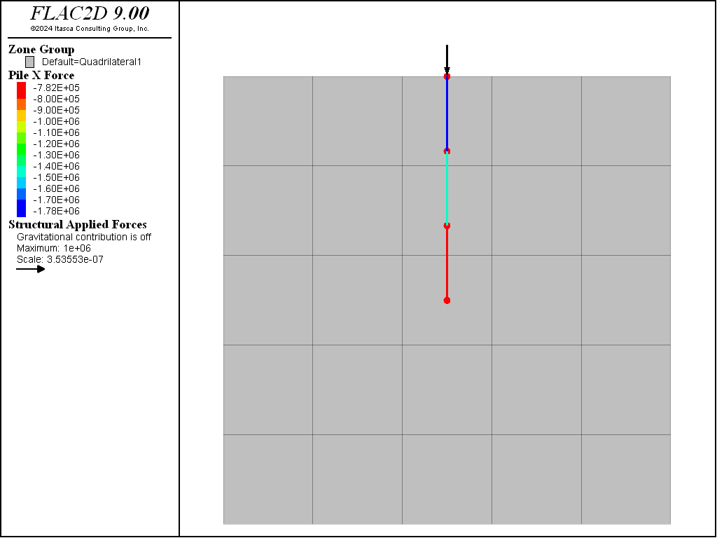
Figure 5: Actual axial forces in vertically loaded piles at 2m spacing (spacing given).

Figure 6: Actual axial forces in vertically loaded piles at 2m spacing (spacing not given).
References
Cook, R. D., D. S. Malkus, and M. E. Plesha. Concepts and Applications of Finite Element Analysis, Third Edition. New York: John Wiley & Sons Inc. (1989).
Cook, R. D., D. S. Malkus, M. E. Plesha, and R. J. Witt. Concepts and Applications of Finite Element Analysis, Fourth Edition. New York: John Wiley & Sons Inc. (2002).
Donovan, K., W. G. Pariseau, and M. Cepak. Finite Element Approach to Cable Bolting in Steeply Dipping VCR Stopes, in Geomechanics Application in Underground Hardrock Mining, pp. 65-90. New York: Society of Mining Engineers (1984).
Type-Specific Information
The following sections describe each type of structural element as well as the nodes and links that are used by the structural elements.
- Cable Structural Elements
- Hybrid Bolt Structural Elements (3D only)
- Beam-Type Structural Elements
- Beam Structural Elements
- Pile Structural Elements
- Shell-Type Structural Elements (3D only)
- Shell Structural Elements (3D only)
- Geogrid Structural Elements (3D only)
- Liner Structural Elements (3D)
- Liner Structural Elements (2D)
- Structural Element Nodes
- Structural Element Links
- General Formulation of Structural-Element Logic
structure Commands & FISH (all)
| Was this helpful? ... | Itasca Software © 2024, Itasca | Updated: Apr 02, 2024 |
