Simple Beam — Two Equal Concentrated Loads — Beam Elements

Problem Statement

Note

To view this project in FLAC2D, use the menu command Help ► Examples…. Choose “Structure/Beam/ConcentratedLoads” and select “ConcentratedLoads.prj” to load. The main data files used are shown at the end of this example . The remaining data files can be found in the project.

A simply supported beam is loaded by two equal concentrated loads, symmetrically placed as shown in Figure 1. The shear and moment diagrams for this configuration are also shown in the figure. The shear force magnitude, \(V\), is equal to the applied concentrated load, \(P\). The maximum moment, \(M_{max}\), occurs between the two loads and is equal to \(P a\). The maximum deflection of the beam, \(\Delta_{\rm max}\), occurs at the center and is given by AISC (1980, p. 2-116) as

(1)\[\Delta_{\rm max}\ =\ {P a \over {24 E I}} (3L^2 - 4 a^2)\]

where:	\(E\)	=	Young’s modulus; and
	\(I\)	=	moment of inertia.

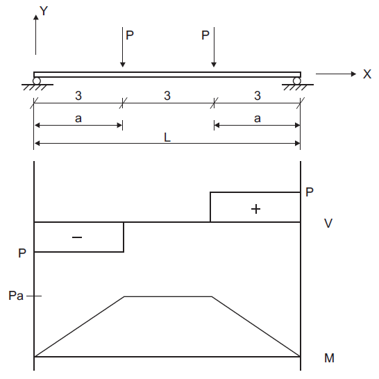
Figure 1: Simply supported beam with two equal concentrated loads (distance in units of meters).

Several properties are used in this example:

Cross-sectional area (\(A\))	0.006 m2
Young’s modulus (\(E\))	200 GPa
Poisson’s ratio (\(\nu\))	0.30
Moment of inertia with respect to the out-of-plane axis (\(I\))	200 × 10-6 m4

Point loads of \(P\) = 10,000 N are applied at the two locations shown in Figure 1.

The FLAC2D model consists of 10 beam elements and 11 nodes, as shown in Figure 2. The beam is created by issuing three separate structure beam create by-line (all with an ID of 1) to ensure that nodes will lie exactly at the beam third points. Also, four elements are created in the middle third to ensure that a node will lie at the exact beam center, so that the displacement of this node can be compared with \(\Delta_{\rm max}\). Boundary conditions corresponding to beam-theory behavior are imposed on all the nodes. Simple supports are specified at the beam ends by restricting translation in the \(y\)-direction. Two point loads acting in the negative \(y\)-direction are applied at the beam third points.

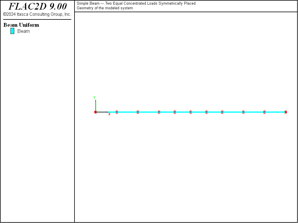
Figure 2: FLAC2D model for simple beam problem.

The displacement field is shown in Figure 3. The maximum displacement occurs at the beam center and equals 6.469×10^-3 m, which corresponds exactly with the theoretical value of equation (1).

An alternative means of visualizing the displacement field for a small-strain simulation is to use the Beam plot item and specify a nonzero value for the deformation factor. Figure 4 shows both the undeformed and deformed shapes.

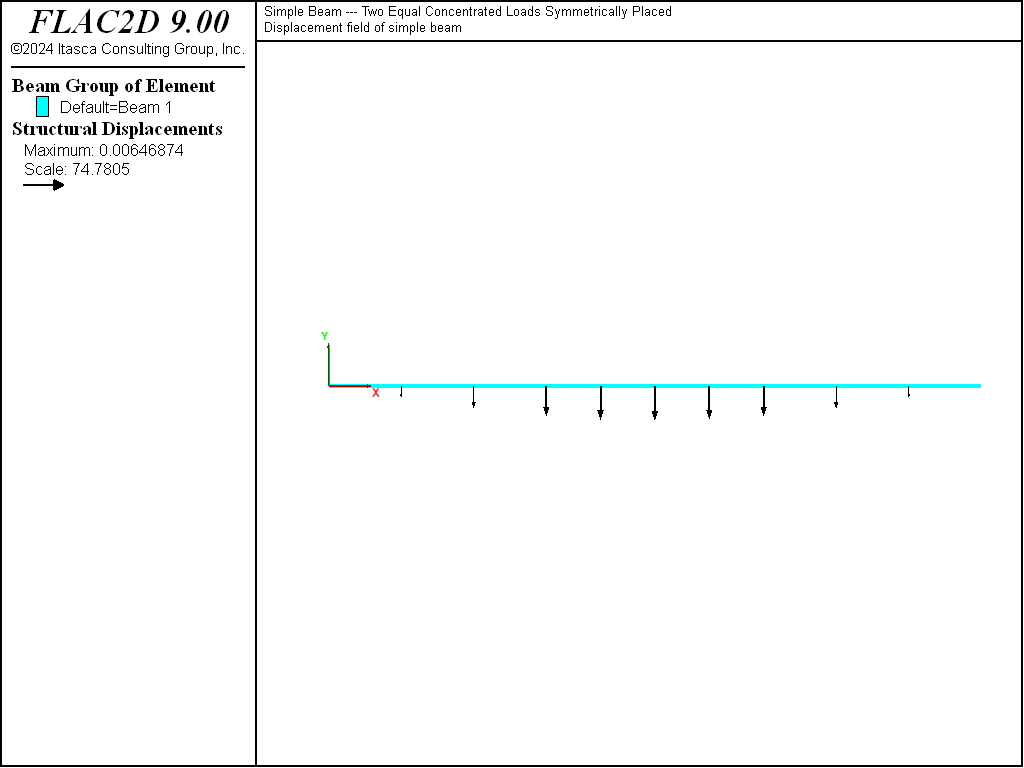
Figure 3: Displacement field of simple beam.

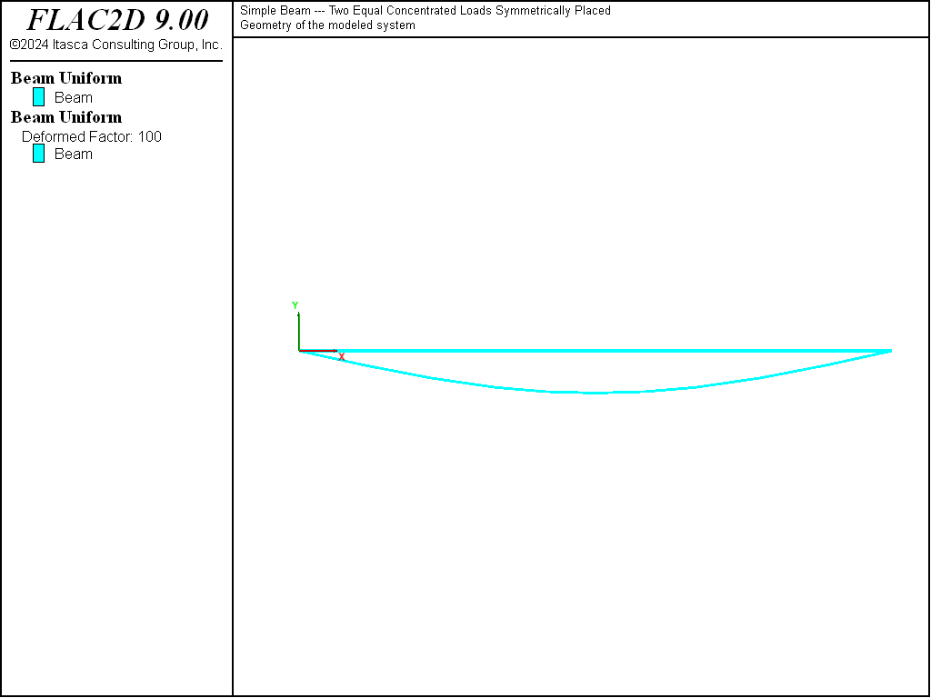
Figure 4: Deformed (deformation factor: 100) and undeformed shapes of simple beam.

Figure 5 and Figure 6 show the shear force and moment distributions, which correspond exactly with the theoretical solutions. These two plot items display these quantities using the force-moment sign convention. In this model, all element systems are aligned with the global system. Thus, the shear force and moment act in the element \(y\)-direction.

The evolution of moment at \(x=1\) is shown in Figure 7 to reach a steady-state value of 10,000 N-m. In this plot, we overlay two histories: one has sampled the moment acting at the right end of element 1 and the other has sampled the moment acting at the left end of element 2. If expressed in a consistent system, these two values should be identical, and the plot demonstrates that they are. This is the case because the elements making up the beam have a consistent orientation (having been created using the structure beam create command). Note that if we print the moment acting on each element in terms of the global system with the command

structure beam list force-node global range component-id 1 2

we find that the moment acting on the right end of element 1 is positive, while the moment acting on the left end of element 2 is negative. This is the correct behavior that satisfies equilibrium.

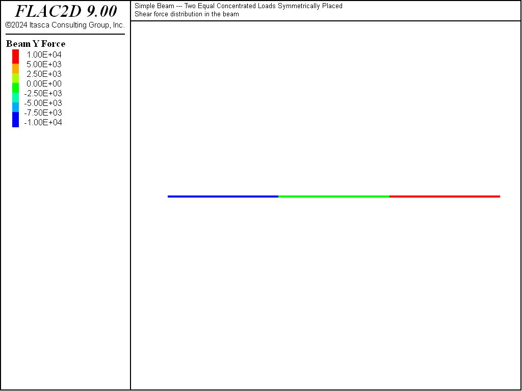
Figure 5: Shear force distribution in simple beam.

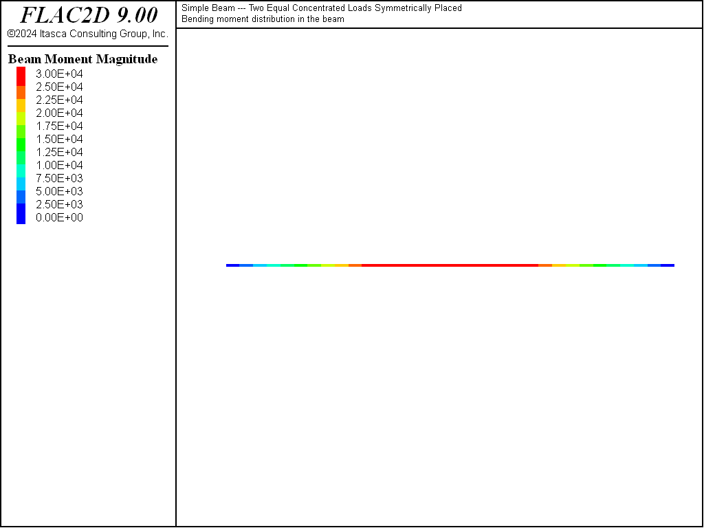
Figure 6: Moment distribution in simple beam.

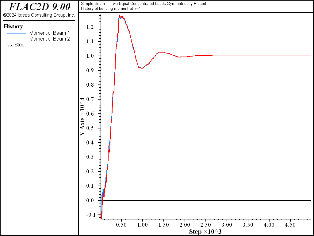
Figure 7: Evolution of moment at x = 1 in simple beam.

Reference

AISC. Manual of Steel Construction, Eighth Edition. Chicago: American Institute of Steel Construction Inc. (1980).

Data File

ConcentratedLoads.dat

model new
model large-strain off
model title ...
      "Simple Beam --- Two Equal Concentrated Loads Symmetrically Placed"
; Create the beams; Ensure nodes will exist at the three points
structure beam create by-line (0,0) (3,0) id=1 segments=3
structure beam create by-line (3,0) (6,0) id=1 segments=4
structure beam create by-line (6,0) (9,0) id=1 segments=3
; Assign beam properties
structure beam property young=2e11 poisson=0.30 cross-sectional-area=6e-3 moi=200e-6
; Specify model boundary conditions (including applied loads)
structure node fix velocity-y range union position-x=0 position-x=9
                   ; apply point loads
structure node apply force=(0.0,-1e4) range union position-x=3 position-x=6 
; Setup histories for monitoring behavior.
structure beam history name='mom1' moment end 2 position (0.5,0) 
                   ; moment, right of element 1
structure beam history name='mom2' moment end 1 position (1.5,0)
                   ;  moment, left of element 2
; Bring the problem to equilibrium
model solve ratio-local=1e-7
model save 'ConcentratedLoads'