FLAC2D Modeling • Tutorials

Tutorial: Quick Start (FLAC2D)

This tutorial steps through the actions necessary to quickly get a first FLAC2D model to solution. Very little time is spent explaining the various user interface elements being used. Rather, the focus is on getting something together and providing basic familiarity with the user interface. A more detailed tutorial is presented next in Tutorial: Illustrative Model — Mechanics of Using FLAC2D, which devotes more explanation to the recommended modeling sequence and the user interface elements involved.

Note that this tutorial can be done with the Demonstration Version of FLAC2D. A valid license is not required.

Help

A user reading this page has found the HTML documentation for FLAC2D. By default, program documentation overlays the i Tools panel to the right in the FLAC2D window. However, it will be easier to proceed through this tutorial by opening this document in another window. To do so, right-click in this document and select Open in Default Browser. The current page of documentation will open in the system default browser. The overlay in FLAC2D may be closed using the button at the top-right. It is helpful to have two screens when walking through tutorials: one for the HTML document and one for FLAC2D.

Sketch

It is assumed, at this point, that FLAC2D is running and the initial setup dialogs have been processed.

Choose File ‣ New Project from the main menu.

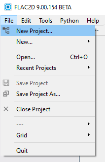
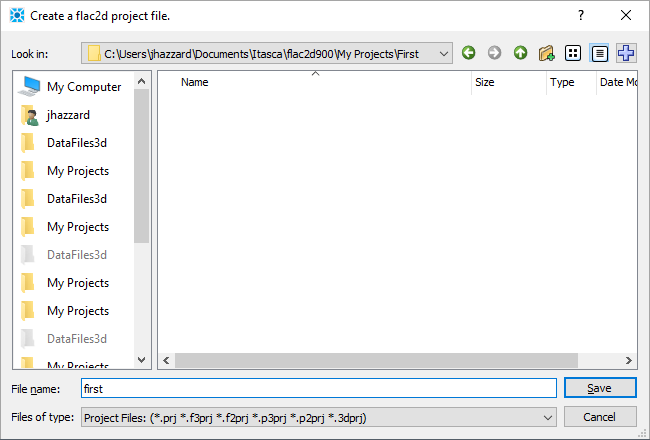
Then save a new project file as “first”.

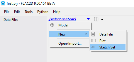
Usually, 2D models start with building the geometry in Sketch. Choose New ‣ Sketch Set from the i content selector in the Sketch workspace.

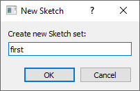
FLAC2D will ask for a name for the new Sketch set. Type “first” as the set name. Then press OK to create the Sketch set.

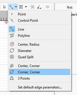
At this point, the set is empty. One could import a dxf or similar to define a geometry, but for this tutorial the geometry is drawn manually. From the drop-down draw tool menu , select the icon of a rectangle defined by Corner, Corner.

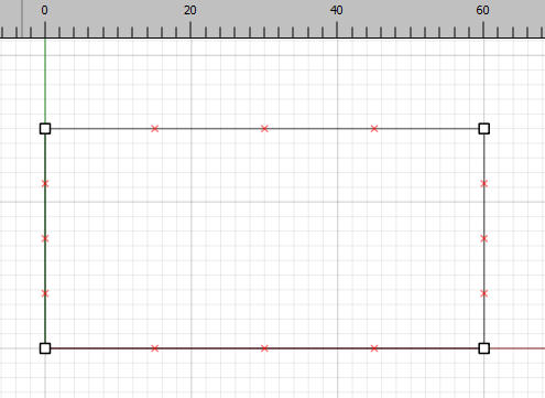
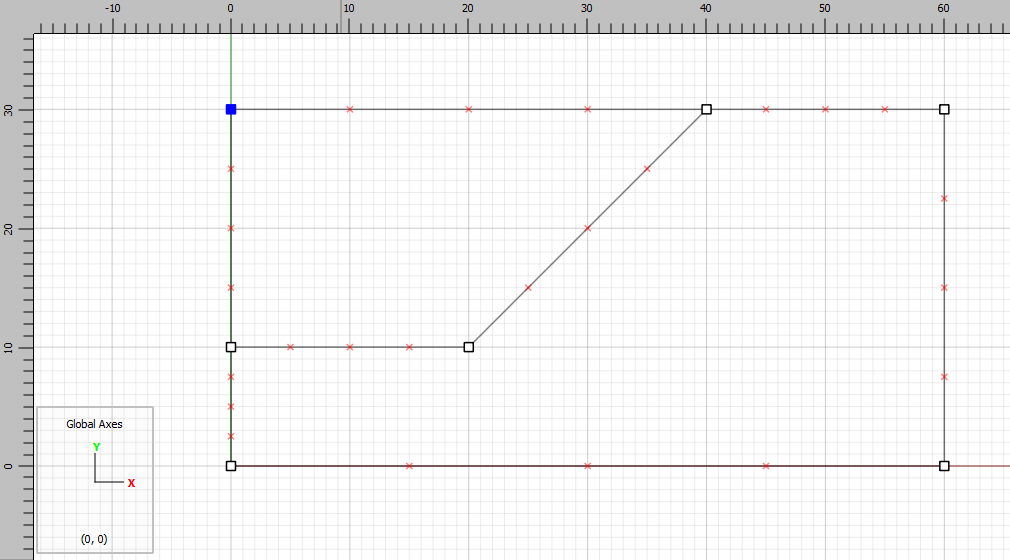
Now a rectangle defined by two points will be drawn. The background grid and coordinate rulers at the top and left side should be visible. The intersection of a vertical green line and horizontal red line denotes (0,0). If (0,0) isn’t visible, use the mouse wheel to zoom in and out.

Guided by the axes and rulers, click on 0,0 for the first point. Then click on 60,30 to complete the rectangle. It should appear as shown.

The rectangle represents the extent of the model. It may be desirable to center and zoom in. Per above, roll the mouse wheel up to zoom in. Press ctrl+R to center or press the reset view button in the View section of the Tools panel.

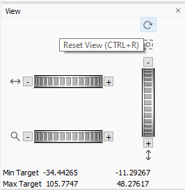
If the Tools panel isn’t visible at right, press the Tools button located near the top right corner of the FLAC2D window.

To pan (move the plot horizontally and vertically), use the controls on the right side or use the mouse buttons. To use use the mouse, first click on the selection tool:

Then hold down the right mouse button, followed by the left mouse button. Moving the mouse will now cause the model to pan.

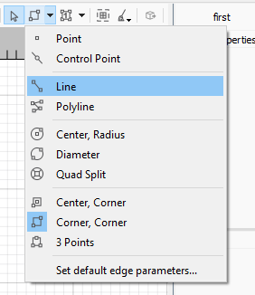
Next two lines are drawn to define the slope. Click on the drop-down Draw tool menu and select Line.

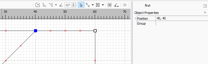
Draw a line from 40,30 to 20,10. Then draw another line from 20,10 to 0,10. The model should look like this:

To correct any mistakes, use the menu command Edit ‣ Undo. Alternatively, click on the Selection tool, click on one of the points, and change its coordinates in the Properties dialog on the right.

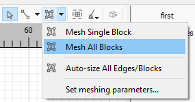
Now that the slope geometry is drawn, it is possible to mesh the model. Red Xs indicate zoning; each X marks the expected placement of a zone edge. To use the default meshing, go the to the Blocking tool and select Mesh All Blocks.

This will create zones as shown.

This is too coarse to be useful. Zone density should be increased. First, get rid of the existing mesh by clicking on the Clean up tools button , and selecting Clean Up Meshes (or, per previous, use the menu command undo).

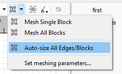
Change the discretization globally by selecting Auto-size All Edges/Blocks () from the drop-down menu on the Blocking Tool menu button .

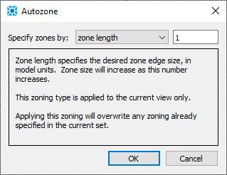
Set the zone length to 1.

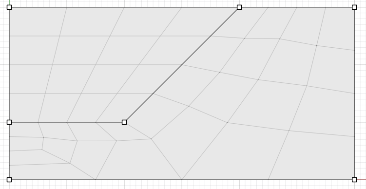
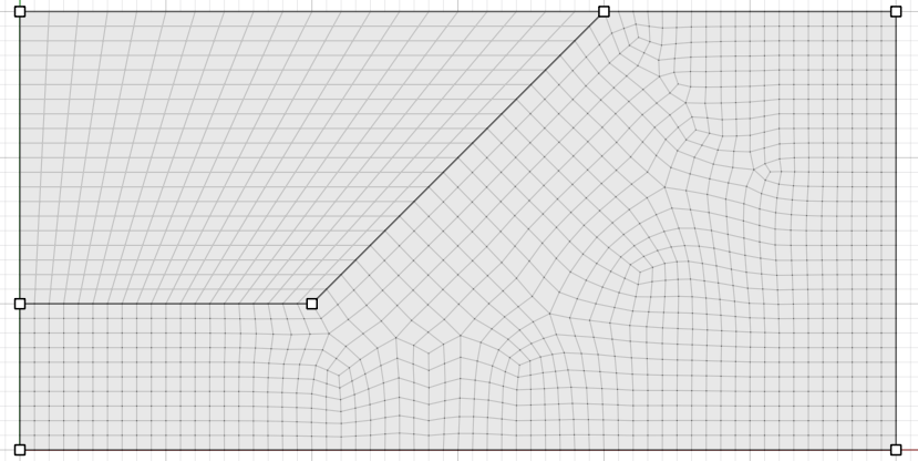
The resulting red Xs indicate increased density of zones on the boundary. To zone the model, go the to the Blocking Tool again and select Mesh All Blocks. The model should appear as shown.

Note

This mesh is a mixture of structured and unstructured mesh. For more information about structured versus unstructured meshes and how to build them, see the topic Meshing in the section covering the Sketch workspace.

Geometry definition and the mesh construction are finished. Click on the Create zones button to create the zones for the FLAC2D model.

Model

The zones are now shown in the Model workspace. This is where zones and faces can be seen, named, and manipulated.

The model should appear something like the image below.

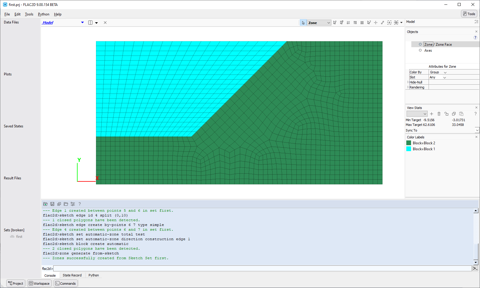
By default, each “block” from the sketch will be assigned a group name—in this case, “Block 1” and “Block 2”. Names may be assigned in the Model worskspace. (The Sketch workspace also allows group assignment, but the Model is more versatile in that it can be used to assign groups to zones that don’t come from Sketch (e.g., an imported grid).)

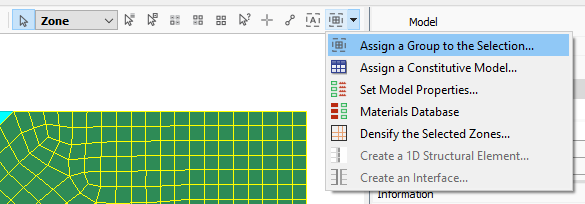
Click on the green block that represents the slope. This selects all of the green zones (selection is indicated with a yellow highlight on zone edges). Click on the drop-down menu next to the Assign menu button and choose Assign a Group to the Selection.

For the group name, enter “Soil”. Leave the slot as “Default”.

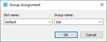
Click OK. Now select the other (light blue) zones and assign them the group name “Air”.

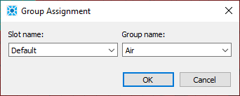
These group names will be used later when identifying different parts of the model.

Note

For more information about groups and slots, see Groups.

Next constitutive models and properties are specified. Select both sections of the model by clicking one, holding down Ctrl, then clicking the other. Alternatively, press Ctrl-a. Click on the drop-down menu next to the Assign menu button and choose Assign a Constitutive Model ….

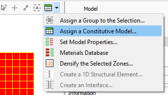
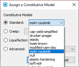
In the resulting dialog, select Standard and choose mohr-coulomb from the drop down menu.

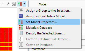
Click Assign. Now, from the Assign menu button, select Set Model Properties ….

In the resulting dialog, fill in the properties as shown.

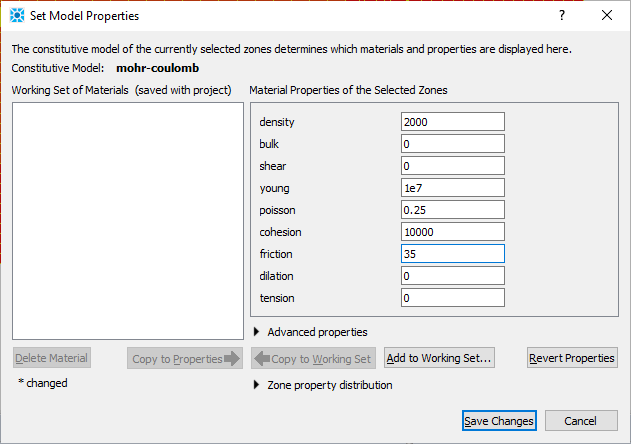
Click Save Changes. The properties are using stress units of Pa. For more information about units in FLAC2D see System of Units.

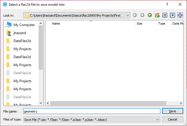
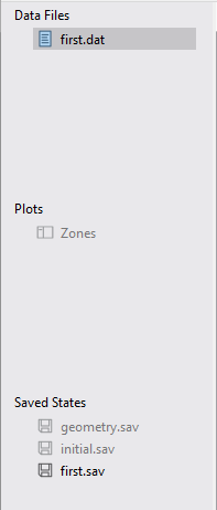
The initial geometry description, the region naming, and the property assignment for the model are complete. It is a good idea to save the model at this point. This will be useful for later reference. Go to File ‣ Save Project. When prompted whether to save the model state, click Yes and save the current model state as “geometry”.

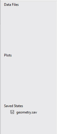
Note that the newly-created save state is now listed in the i Project panel at left.

At this point, the i State Record tab in the Commands area could be used to create a data file, which in turn could be used to recreate this state whenever necessary. For many purposes, however, it is sufficient to use the save file directly, which is how this simple example will proceed.

Data File

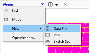
Further development of the model will require constructing a data file. FLAC2D models are entirely command-driven, although, as is seen above, for some commands there are interactive operations in the user interface that can be used to emit the commands. To work on a new data file, go to the content selector at the top left of the workspace (currently it should say “Model”). Then select New ‣ Data File menu entry.

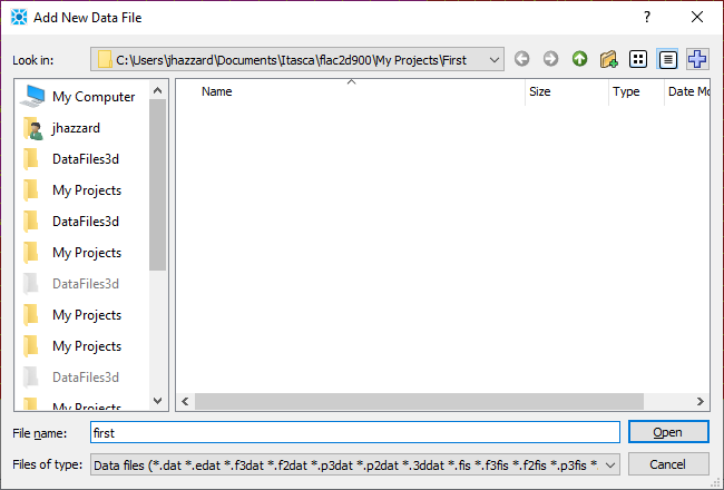
In the ensuing dialog, create a new data file called “first”.

Note

Access the inline help facility by pressing Ctrl+spacebar, or activate context sensitive help by pressing F1, or a combination of both, at any time while generating commands in the editor.

The first command in this data file restores the geometry model state just created as a starting point using the model restore command. Type (or copy and paste from this document) the following line at the top of the editor. (From this point forward, continue typing or copy-pasting the command listings in the gray boxes, as they appear, into the data file.)

model restore "geometry"

The constitutive model and properties have already been assigned. Now the boundary conditions for the model are given. In this case the model will have roller boundaries on the sides and the bottom fill be fixed. The top will be left free. Boundary conditions are typically assigned using the zone face apply command. Roller boundaries are created using the velocity-normal keyword of the command. A fixed boundary can be simulated by specifying that both components of velocity are 0.

; Boundary Conditions
zone face apply velocity-normal 0 range position-x 0
zone face apply velocity-normal 0 range position-x 60
zone face apply velocity 0 0 range position-y 0

Next, it is necessary to assign initial conditions. For this simple case, this is only stresses due to gravity, so gravity is assigned using the model gravity command. Stresses due to gravity are initialized with the zone initialize-stresses command.

; Initial Conditions
model gravity 9.81
zone initialize-stresses

Next, the analysis is set to small strain (see the topic Large Strain/Small Strain) and the model is solved to reach initial equilibrium. Because the internal zoning is somewhat irregular, the zone initialize-stresses command comes close to equilibrium but is not perfect. Solving the model is necessary to reach complete equilibrium. Because the model is already close, this takes little time. After reaching equilibrium, the state is saved with the name initial to serve as a starting point for future changes.

model large-strain off
model solve
model save "initial"

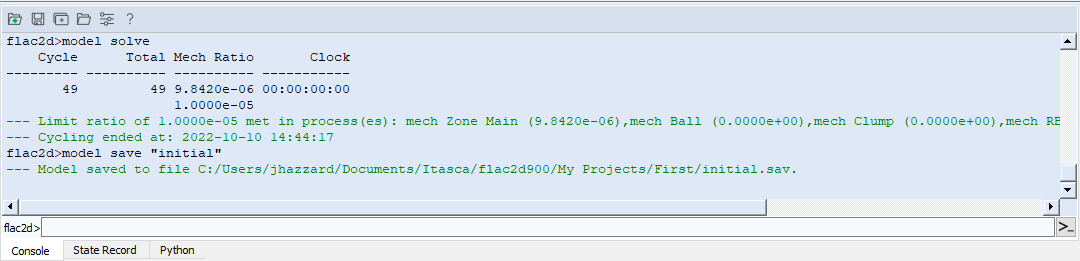
To run the data file, click on the green arrow at the top left . Calculation progress is shown in the Console tab in the Commands area. Users may see slightly different numbers of steps due to the randomness of the mesh creation.

In a larger FLAC2D project, it would be practical to start a new data file with model restore "initial", so the investigation could continue without having to repeatedly create an initial equilibrium state. This example—which is relatively small and fast—simply continues construction of the model from a single data file.

The next step is to excavate the slope. While this could be done by immediately removing the zones (either by changing to the null model using zone cmodel assign null or by deleting the zones using zone delete), it is better practice to excavate the zones gradually so quasi-inertial effects do not exaggerate the failure as a result of excavation. This is done using the zone relax excavate command as follows.

; Excavate Slope
zone relax excavate range group "Air"

Note

Recall that the group name “Air” was previously specified in the Model workspace.

Following that, the model is solved to equilibrium again and the final model state is saved. Enter the following lines and click the Execute button again the run the model.

; Solve to equilibrium after excavation
model solve
model save "first"

The complete resulting data file should look like this:

model restore "geometry"

; Boundary Conditions
zone face apply velocity-normal 0 range position-x 0
zone face apply velocity-normal 0 range position-x 60
zone face apply velocity 0 0 range position-y 0

; Initial Conditions
model gravity 9.81
zone initialize-stresses

; Solve to initial equilibrium
model large-strain off
model solve
model save "initial"

; Excavate Slope
zone relax excavate range group "Air"

; Solve to equilibrium after excavation
model solve
model save "first"

If there are any errors, an error message will appear in a dialog and the line will be highlighted in the editor. Just repair the problem (using this tutorial as a reference if necessary) and press the Execute button again.

Plotting

From the content selector, select New ‣ Plot.

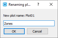
Name the plot “Zones” and click OK.

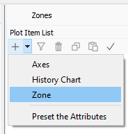
An empty plot is shown. In the Tools panel at right, click on the down arrow next to the Build Plot tool button ( ), and select the Zone entry.

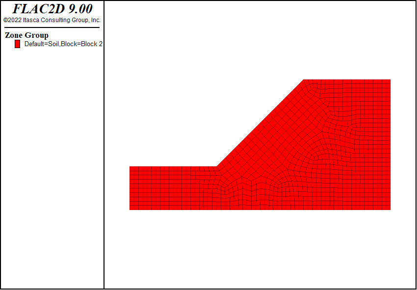
After right-clicking and dragging to look around, and using the mouse wheel to zoom in and out, the initial plot should appear something like the following.

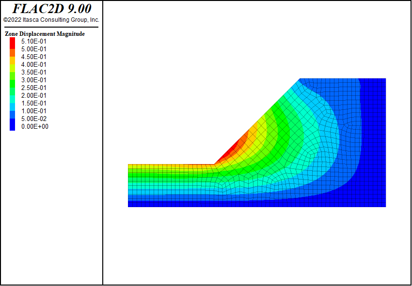
To see model results, go to the Attributes section in the Tools panel. Choose Contour in the Color By attribute. The default quantity should be Displacement.

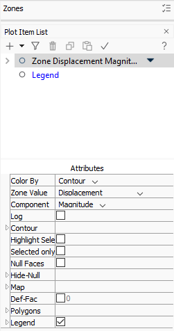
This should give a result similar to the one shown below.

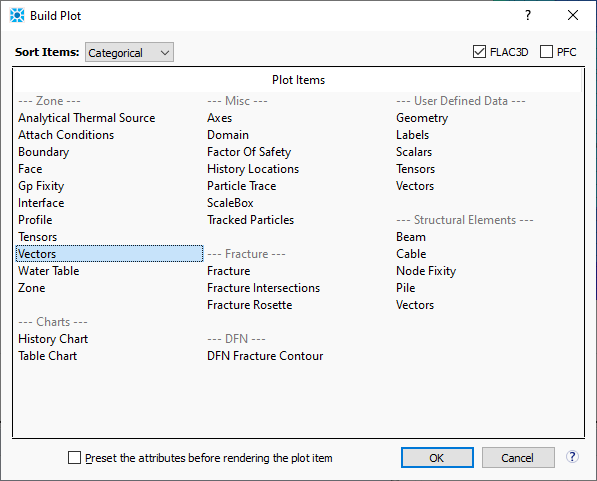
This shows the magnitude of displacement. To see the direction, add vectors by selecting the Build Plot tool button ( ) and choosing Vectors under the Zone heading.

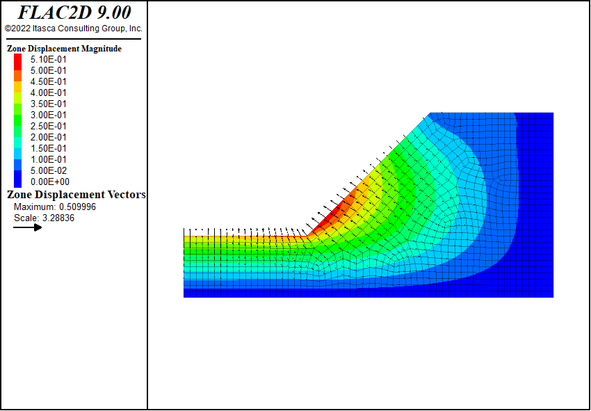
The model should appear like this:

The extent of failure is seen by first selecting the “Zone Displacement Magnitude” plot item from the plot item list, and then selecting Label again from the Color By attribute, followed by State from the Label attribute.

This should result in a plot that looks like the one below.

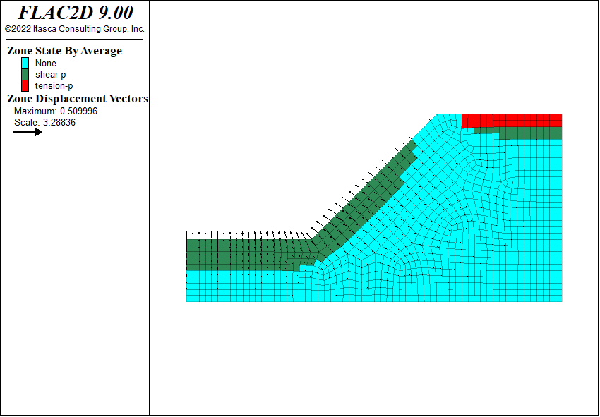
There has been shear failure in the past (green zones denoted by shear-p) and tension failure in the past (red zones denoted by tension-p), but there is no current failure, and the slope is stable.

Factor of Safety

The factor of safety for this slope can be easily calculated with the command model factor-of-safety. Go back to the data file by double-clicking on “first.dat” in the Project panel.

Add this line to the end of the data file:

model factor-of-safety

Hit the Execute button to run the model. This may take a couple of minutes. When it is finished, three new save states have been created:

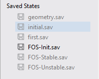
The first is the initial state, the second is just stable and the third is just failing. Double-click on “FOS-Unstable.sav” to restore this state. Double-click on the “Zones” plot in the Project Pane to show the plot again.

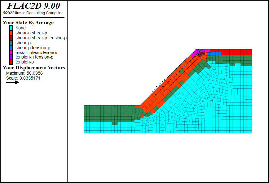
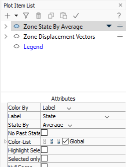
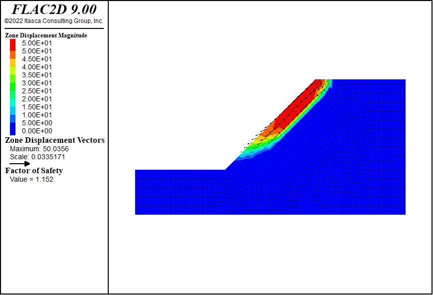
There are now zones failing in shear (shear-n) and tension (tension-n). There is also significant displacement. To view the displacement contours, click on the “Zone State By Average” plot item and select Contour from the Color By attribute.

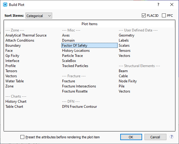
The calculated factor of safety is displayed in the console, but it can also be added to the plot. Select the Build Plot tool button ( ) and choose Factor of Safety under Misc.

The plot should now appear as shown. The plot legend indicates that the calculated factor of safety is 1.152.

At this point, save the project by selecting File ‣ Save Project on the main menu. Note that the project file stores the plot(s) that have been created. These are not part of the model states (save files).