Massflow Tutorial

Problem Statement

Note

To view this projects in MassFlow, use the menu command Help ► Examples…. Choose “MassFlow/ Examples/ Tutorial/ ” and select tutorial.prj. The data file used is shown at the end of this example. All data and input files are found in the project directory.

This tutorial describes how to build a simple model, run it, and view the results. This tutorial is designed to be run with the demo version, so a license is not required.

MassFlow is a command-driven program. Those commands can be issued from the command prompt, or, more commonly, in a data file. The data file is essentially a list of commands that can be issued and processed in unbroken sequence. This is both more efficient than either the command prompt or mouse/keyboard commands—either of which is limited to issuance of one command at a time—and has the added advantage of being able to provide a readable representation of a problem from beginning to end. One or more data files are usually stored in a Project. Creating a new project and adding data files to it is described next.

Create a New Project

Create a project for this tutorial.

1. Choose File ‣ New Project… from the main menu.

2. Navigate to the folder where the project file will be saved.

3. Name the project “tutorial” in the File Name field.

4. press Save or press Enter .

Create a Data File

For this tutorial, a single complete data file for the problem will be created.

1. Select File ‣ New Data File… or press Ctrl + N.

2. At the “File Name” field, enter “tutorial”.

3. Press Save or press Enter .

Note the new data file is made the active pane.

Refer to the Projects section for complete information on working with projects.

New Model

Start by typing the following lines into the data file, or copy and past from the listing below:

model new
model random 10000

The model new command clears the model state. It is not neccesary at this time since there is nothing in the model yet, but it is useful to have at the top of the file in case you run the data file again and you want to start fresh. The model random command sets a random seed that is used when randomly generating marker locations. This is generally not necessary, but is used here so that you get exactly the same results as shown in the plots below. Using a different random seed will result in slightly different marker distributions.

Mine Blocks

Every massflow model requires the definition of mine blocks. These define the geometry of the mine, the material properties, ore grade, caving times etc. Mine blocks are creating by importing from a tab-delimited ASCII text file. The file format is described in the command massflow mineblock import.

For this tutorial, a file is provided (mineblocks.txt) with all of the mandatory data and 10 extra ore properties. To import the mine blocks, follow these steps:

1. Type the lines below into the “tutorial.dat” data file (or you can copy and paste them directly from the listing below). Note: you can use massflow mine-block import “mineblock.csv” if your data is in comma-delimited format. If so, only a first line header is required and the block model properties start from the second line.

; mine blocks
;massflow mine-block import-txt "mineblocks.txt"

2. Press the Execute button ( ). The commands are processed and echoed in the Console pane output.

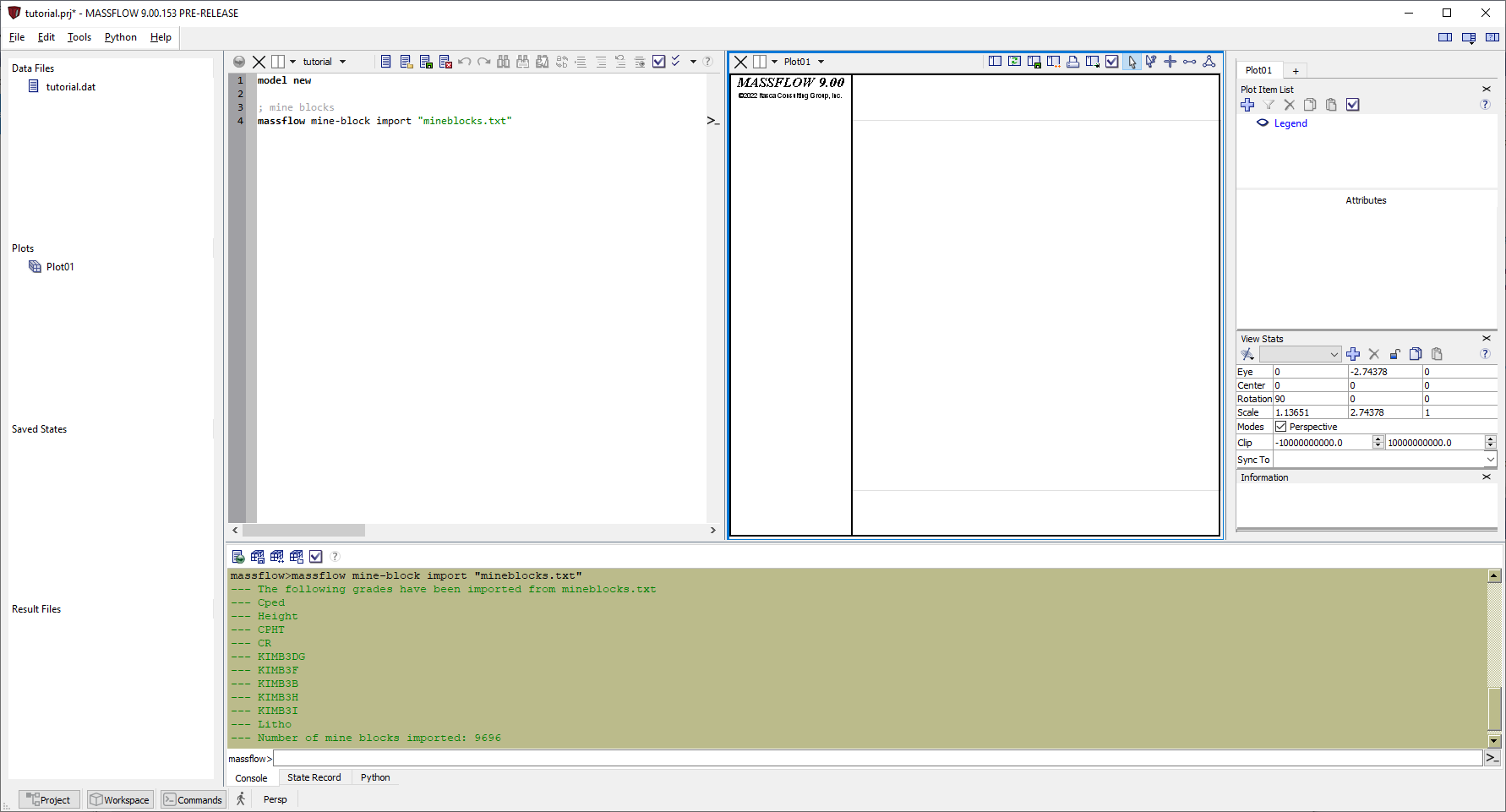
After importing the file you will see the list of imported ore properties in the Console window. We can now plot the mine blocks.

First it is useful to split the window so we can see the data file and the plot. Click on the drop-down arrow next to the Tiled Viewer icon and choose Split right.

In the right window, click the drop-down arrow next to the Select Document to View icon. Select New ‣ Plot

Use the default name, Plot01, and click OK. Your screen should now look like this:

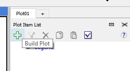
Click on the plot window on the right (it should now be highlighted with a blue border as shown above). In the Control Panel on the right-hand side, click on the Build Plot tool button ( ).

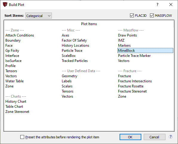
From the list of plot items, under MassFlow select MineBlock.

Use the right mouse button to rotate and the mouse wheel to zoom. To pan, hold down first the right mouse button and then the left. After rotating and panning to look around, the initial plot should appear something like the following.

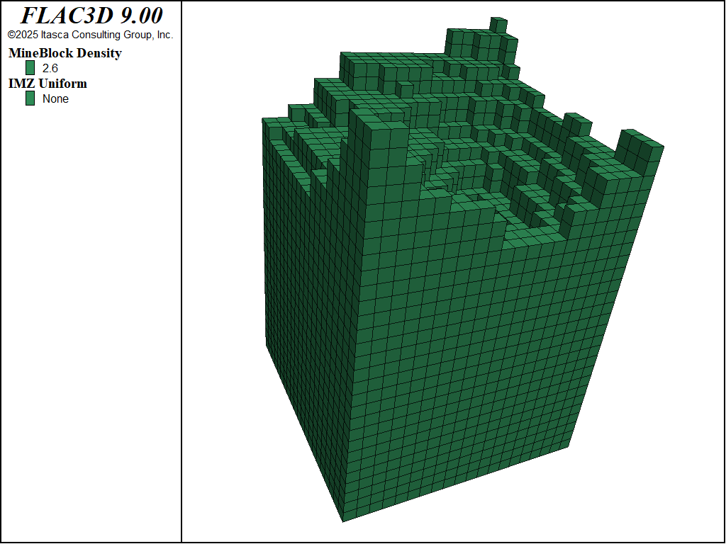
Figure 1: Mineblocks colored by density before the analysis.

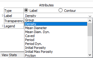
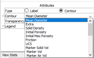
By default, the mine blocks are colored by density. In the Attributes section of the Control Panel, click in the drop down labeled Label to see what other quantities may be selected for coloring the blocks.

You can also choose Contour in the Type attribute to plot add contours, rather than solid colors.

Draw Points

Draw point names, locations, and drawbell shapes are also imported from a file. The file format is described in the command massflow drawpoint import.

The drawbell shapes are defined in a separate file as described in massflow drawpoint import-drawbell.

The import is done by adding these two lines to the data file and then clicking the Execute button ( ):

; draw points
;massflow drawpoint import-txt "drawpoints.txt"

Note: you can use massflow drawpoint import “drawpoints.csv” and massflow drawpoint import-drawbell “drawbells.csv” if your data is in comma-delimited format.

The drawbells can be plotted by again clicking on the Build Plot tool button ( ) and selecting MassFlow - DrawPoints. You can’t see them because they are inside of the mine blocks. Hide the mine blocks by clicking on the eye icon next to the MineBlock plot item in the Plot Item list.

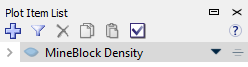
When the mineblocks are hidden, you can zoom in to see the drawbells.

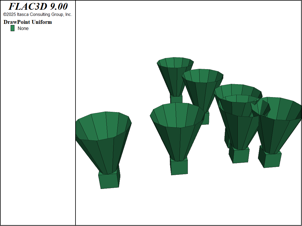
Figure 2: Drawbells for this example.

Next, import the draw schedule using the command massflow drawpoint import-drawperiod. The duration of each draw period and the tonnage extracted during each period is specified for each draw point.

;massflow drawpoint import-drawbell-txt "drawbells.txt"

Note: you can use massflow drawpoint import-drawperiod “drawperiods.csv” if your data is in comma-delimited format.

Markers

Markers are points in space that move during the caving operation. By monitoring the marker movements, you can understand the rock behavior suring caving.

First you need to specify the marker spacing as a percentage of the mine blocks size. If a spacing is not given, a value of 0.25 is assumed.

MassFlow can be set up to print marker information to a file at specified time intervals. As with the save files, the interval can be given in terms of days or periods. In this example, we will specify a report to be generated every 10 periods. Since a period is 7 days (from the imported drawpoint schedule file), then a report will be written for every 7 days of extraction.

Finally, it is possible to specify the locations of one or more marker points to monitor the movement during the caving operation. This can be done by importing locations from a file (see massflow import-trace), or by giving commands directly (see massflow marker trace). In this example, we will import a file to specify 4 trace locations as shown below. The file simply contains rows of x, y, z coordinates. The movement of these specified points can then be plotted later as “traces”.

The marker setup is done with the following commands:

massflow drawpoint import-drawbell "drawbells.csv"
massflow drawpoint import-drawperiod "drawperiod.csv" 

; markers

Record

You can record the mass for each period at each drawpoint using the massflow record: command. You can also record the cumulative mass over the whole simulation. In addition, the mass associated with each user-defined ore unit can be recorded. In this example, we record the period mass and cumulative mass for all drawpoints summed together using the following commands:

massflow marker report-period 10
massflow marker import-trace "tracemarkers.txt"

Initialize

Various computation parameters are then set using the command massflow initialize. Default values exist for many parameters, but as a minimum, the user must set the number of days or periods for which you’re going to solve, and the interval between save states.

The command below will set up the model to run for 500 days, saving the state every 100 days, with a marker spacing of one-quarter of the mine block size.

Once everything is finalized, the command massflow clean must be given to set up all of the necessary data structures.

massflow record name 'all DPs' cumulative true
massflow record name 'DP1' drawpoint 'DP1' cumulative true

Compute

The massflow compute command will start the computation. After this add a command to save the final state as shown below.

massflow initialize compute-days 500 save-days 100
massflow clean

Press the Execute button ( ) to run the whole analysis. The progress will be printed in the control panel. It will take a few minutes to perform the computation, depending on the speed of your computer.

It is possible to watch the markers move as the calculation progresses. Click on the Plot01 tab and add MassFlow - Marker. Zoom out (or press CTRL-R to reset the plot) and you will see all of the markers. By default, they are colored by type.

Figure 3: Markers colored by type at the end of the analysis.

Analysis

After finishing the computation, the markers should appear as shown in Figure 3. By double-clicking on different save states on the left side under Saved States you can observe the changing nature of the markers over time.

The markers at 200 days are shown in Figure 4.

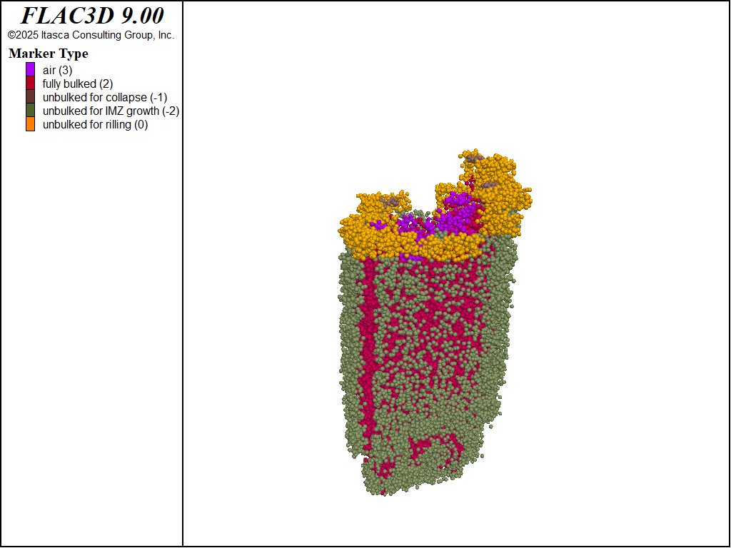
Figure 4: Markers colored by type after 200 days.

More details about the markers can be obtained from the reports that were automatically generated during computation (with an interval specified by the massflow marker report-period command. The files are tab-delimted text files with names indicating the day of extraction (e.g. markersDay70.txt). These files contain detailed information about the markers at each interval (MORE HERE).

As well as detailed information about all of the markers, we can plot the trajectory of the specific markers tracked as trace markers. Double-click on massflowDay0040.sav in the Saved States. Go to Plot01, and add the plot item Particle Trace MArker. Hide other plot items if necessary to see the traces. You should see a plot like Figure 5. The trajectories are contoured by time so you can see the eveolution of movement of the selected marker points.

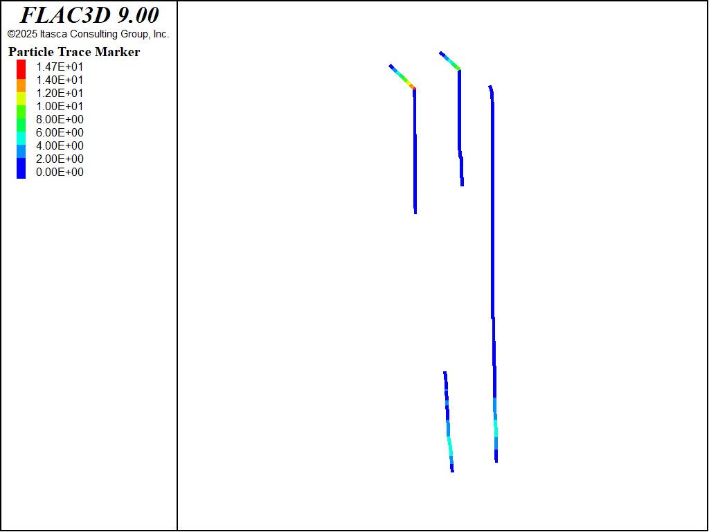
Figure 5: Marker traces at the end of the analysis.

Details about the traces can also be written to a file with the command massflow marker trace-report.

Extraction and IMZ

Details about the extracted mass can be obtained with the command massflow drawpoint extraction-report.

The Isolated Movement Zones can be plotted by adding the IMZ plot item. If you hide the mine blocks and the markers, but show the draw points, you should see a plot like Figure 6. You can change the color of the drawpoints by selecting the DrawPoint plot item, under Label - Color List, click on the green squre and choose another color.

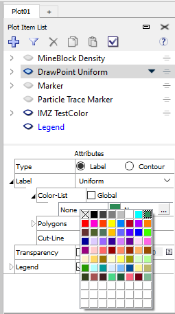
To make viewing easier, you can also make the IMZs transparent by selecting the IMZ plot item and checking the box for Tranparency

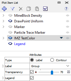
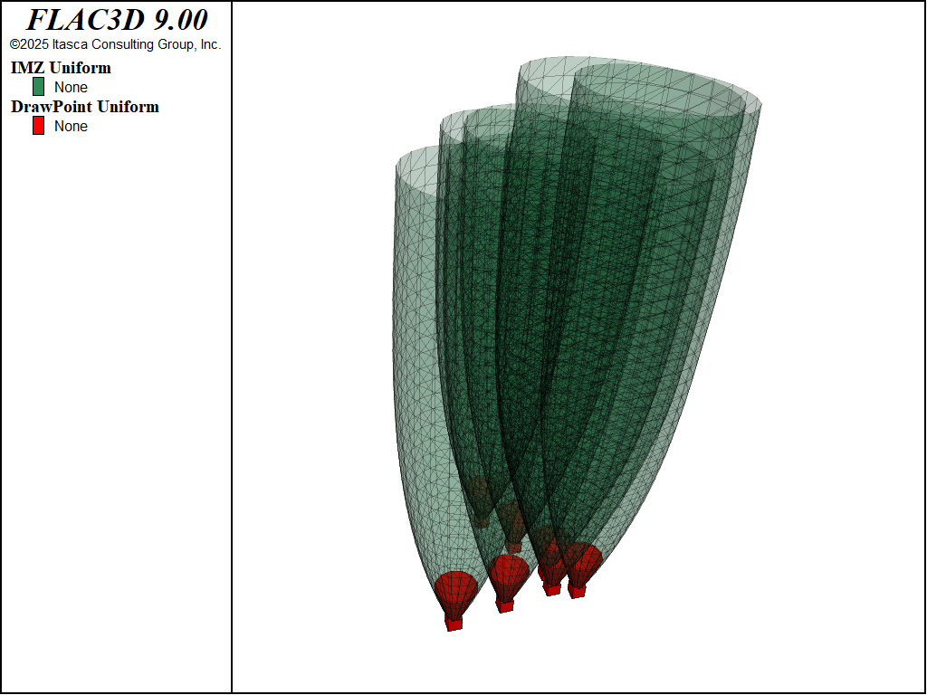
Figure 6: IMZs at the end of the analysis.

Mass Records

The mass extracted by all of the drawpoints by period and cumulative are plotting in Figure 7. This plot was created by choosing Charts - Table Chart from the plot items. The axis titles were modified in the Table plot item attributes.

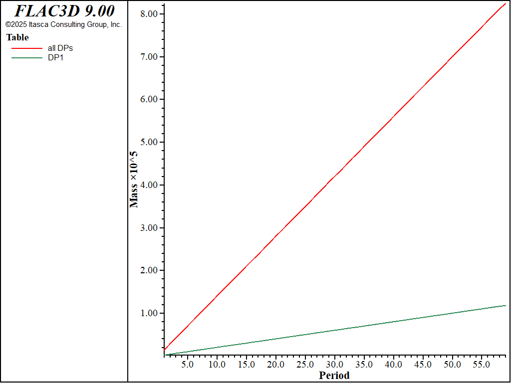
Figure 7: Extracted mass for all of the drawpoints.

Size Distribution

It is possible to generate a plot of fragment size distribution for extracted markers from different periods, or over the duration of the simulation. See massflow marker-size-distribution. Type the following line into your data file:

You don’t want to run the whole analysis again, so highlight the line, right click, and select Run Selection. This will generate a table that holds the size distribution data.

Create a new plot and call it Size Distribution. Click the Build Plot tool button ( ) and select Table. In the attributes for the table, click on the + next to size-distriution. You should now see a curve of cumulative % passing versus fragment diameter. Change the x-axis to be a log scale by expanding the Axis-1 attribute and clicking the Log checkbox. Here you can also change the label (for example, Fragment Diameter). Similarly for Axis-2 you can change the Label to % Passing. You can also change the number display on Axis-2 by unchecking the Auto box under Exponent, changing the Value to 0, and then unchecking the Exponent box. Finally, you can change the color of the line by explaning the Seried entry and selecting a different color for the line. Your Attributes should now appear as shown below, and the resulting table plot is shown in Figure 8.

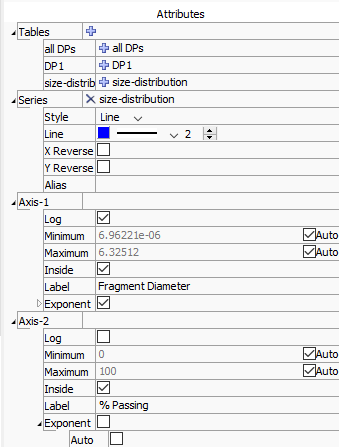
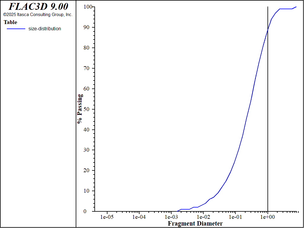
Figure 8: Size distribution of the extracted drawpoints.

Data File

tutorial.dat

model new
model random 10000

; mine blocks
;massflow mine-block import-txt "mineblocks.txt"
massflow mine-block import "mineBlocks.csv"

; draw points
;massflow drawpoint import-txt "drawpoints.txt"
;massflow drawpoint import-drawbell-txt "drawbells.txt"
;massflow drawpoint import-drawperiod-txt "drawperiods.txt" 
massflow drawpoint import "drawpoints.csv"
massflow drawpoint import-drawbell "drawbells.csv"
massflow drawpoint import-drawperiod "drawperiod.csv" 

; markers
massflow marker initialize spacing 0.25 
massflow marker report-period 10
massflow marker import-trace "tracemarkers.txt"

; record masses in tables
massflow record name 'all DPs' cumulative true
massflow record name 'DP1' drawpoint 'DP1' cumulative true

; initialize
massflow initialize compute-days 500 save-days 100
massflow clean

; compute
massflow compute 
model save "massflow.sav"

massflow marker trace-report
massflow drawpoint extraction-report

massflow marker size-distribution