FLAC3D Modeling • Introduction

Overview

FLAC3D is a three-dimensional explicit Lagrangian finite-volume program for engineering mechanics computation. The basis for this program is the well-established numerical formulation used by our two-dimensional program, FLAC.[1] FLAC3D extends the analysis capability of FLAC into three dimensions, simulating the behavior of three-dimensional structures built of soil, rock, or other materials that exhibit path-dependent behavior.

Materials are represented by polyhedral elements within a three-dimensional grid that is adjusted by the user to fit the shape of the object to be modeled. Each element behaves according to a prescribed linear or nonlinear stress/strain law in response to applied forces or boundary restraints. The material can yield and flow, and the grid can deform (in large-strain mode) and move with the material that is represented.

The explicit, Lagrangian calculation scheme and the mixed-discretization zoning technique used in FLAC3D ensure that plastic collapse and flow are modeled very accurately. Because no matrices are formed, large three-dimensional calculations can be made without excessive memory requirements. The drawbacks of the explicit formulation (i.e., small timestep limitation and the question of required damping) are overcome by automatic inertia scaling and automatic damping that minimizes effects on the path to failure. FLAC3D offers an ideal analysis tool for the solution of three-dimensional problems in geotechnical engineering.

FLAC3D is designed specifically to operate on Microsoft Windows systems and is currently supported on Windows 7, Windows 8, and Windows 10. Calculations on realistically sized three-dimensional models in geo-engineering can be made in a reasonable time period. For example, a model containing 125,000 zones of a Mohr-Coulomb material can be generated within 600 MB RAM. The runtime to perform 5000 calculation steps for a 10,000 zone model of Mohr-Coulomb material is roughly 30 seconds on a 3.2 GHz Intel 6-Core i7 CPU.[#f2]_ The number of calculation steps required to reach a solution state with the explicit-calculation scheme can vary, but a solution typically can be reached within 3000 to 5000 steps for models containing up to 10,000 elements, regardless of material type. (The explicit-solution scheme is explained in the Theoretical Background section.) With the advancements in floating-point operation speed and the ability to install additional RAM at low cost, it should be possible to solve increasingly larger three-dimensional problems with FLAC3D.

The FLAC3D program interface includes both command-line (CLI) and graphical (GUI) capabilities. All aspects of program operation are available via the CLI in the Console pane. Many but not all program operations can be performed in the program’s GUI components. Some operations (plotting, working with extrusions or building blocks, etc.) will be comparatively easier in the GUI components, and others may be invoked more efficiently (or necessarily) at the command line. Many FLAC3D commands will be similar or identical to those found in the Itasca program PFC, and both programs share a common command syntax and structure.

FLAC3D features accelerated 3D graphics that allow for rapid model visualization. Extensive plotting capabilities—including easy mechanisms for constructing animations (movies)—are available to facilitate pre- and post-processing.

A comparison of FLAC3D to other numerical methods, a description of general features and updates in FLAC3D Version 6.0, and a discussion of the program’s fields of application are provided in the topics that follow. If you wish to try FLAC3D right away, the best place to start is with the Tutorials.

The Lagrangian Finite Volume Grid

The Lagrangian finite volume grid spans the physical domain being analyzed. The smallest possible grid that can be analyzed with FLAC3D consists of only one zone. Most problems, however, are defined by grids that consist of hundreds, thousands, or millions of zones.

One FLAC3D zone is a hexahedron with eight vertices and six quadrilateral faces. Four other zone types are available (wedge, pyramid, d-brick, and tetrahedron), as degeneracies of this basic zone using fewer vertices and faces. See Zone for a discussion of zone data and conventions, and Theoretical Background for the theory, formulation, and implementation details.

The FLAC3D grid is specified in terms of global x-, y-, and z-coordinates. All gridpoints and zone centroids are located by their (\(x,y,z\)) position vector. A simple cubic grid is shown in the figure below. A set of ready-made (templatized) grids can be accessed from the File ‣ Gridmenu option.

Every gridpoint and zone is identified by an identification number (ID), which can be used as a handle to refer to that specific object.

Grid generation with FLAC3D involves adjusting and shaping the mesh to fit the shape of the physical domain. The generation process may be performed in a variety of ways, such as using commands that build zones from primitive shapes, using the program’s interactive extrusion or building blocks facilities, or using advanced mesh generation techniques with third-party tools.

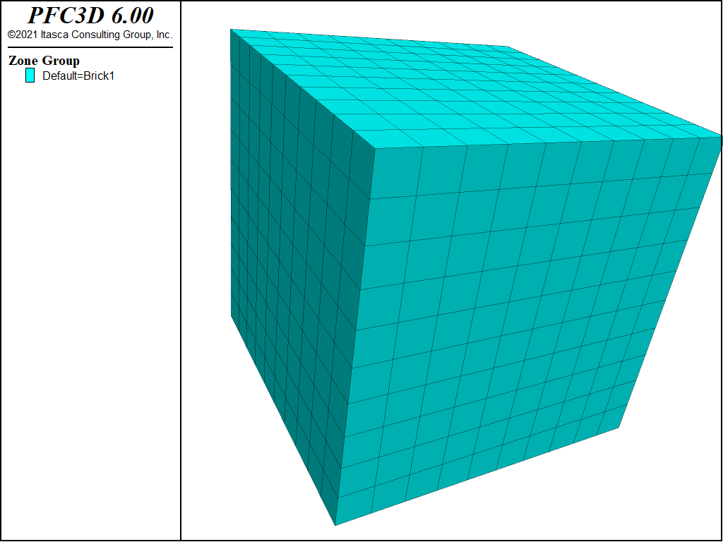
Figure 1: Finite difference grid with 1000 zones.

section on nomenclature formerly appeared here; moved to master glossary

Endnotes

[1]	Itasca Consulting Group Inc. FLAC (Fast Lagrangian Analysis of Continua), Version 8.0, 2014. .. [#f2] See [need a link here to runtime comparison]

[2]

In some finite element (FE) literature, there is the mistaken notion that a dynamic solution method cannot produce a true equilibrium state, compared to an FE solution, which is believed to perfectly satisfy the set of governing equations at equilibrium. In fact, both methods only satisfy the equations approximately, but the level of residual errors can be made as small as desired. In FLAC3D, the level of error is objectively quantified as the ratio of unbalanced force at a gridpoint to the mean of the set of absolute forces acting at the gridpoint. This measure of error is very similar to the convergence criteria used in FE solutions. In both cases, the solution process is terminated when the error is below a desired value.