
Dynamic Modeling Considerations
There are three aspects that the user should consider when preparing a FLAC3D model for a dynamic analysis: 1) dynamic loading and boundary conditions; 2) wave transmission through the model; and 3) mechanical damping. This section provides guidance on addressing each aspect when preparing a FLAC3D data file for dynamic analysis. Solving Dynamic Problems and Verification Problems illustrate the use of most of the features discussed here.
Dynamic Loading and Boundary Conditions
FLAC3D models a region of material subjected to external and/or internal dynamic loading by applying a dynamic input boundary condition at either the model boundary or internal gridpoints. Wave reflections at model boundaries may be reduced by specifying quiet (viscous) or free-field boundary conditions. The types of dynamic loading and boundary conditions are shown schematically in Figure 1; each condition is discussed in the following sections.
Application of Dynamic Input
In FLAC3D, the dynamic input can be applied in one of the following ways:
- an acceleration history;
- a velocity history;
- a stress (or pressure) history; or
- a force history.
Dynamic input is usually applied to the model boundaries with the zone face apply
command. Accelerations, velocities, and forces can also be applied to interior gridpoints by
using the zone gridpoint fix command. Note that the free-field boundary, shown in
Figure 1, is not required if the only dynamic source is within
the model (see Free-Field Boundaries).
The history function for the input is treated as a multiplier on the value specified with the
zone face apply command. The history multiplier is assigned with the history
keyword and can be in one of two forms:
- a table defined by the
tablecommand; or- a FISH function.
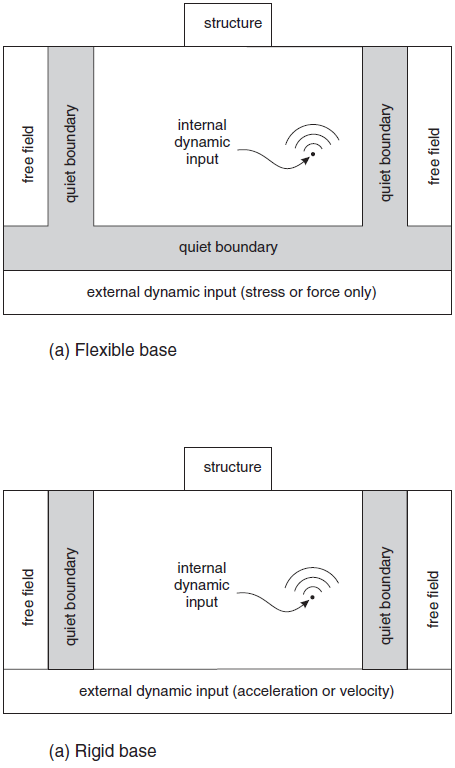
Figure 1: Types of dynamic loading and boundary conditions available in FLAC3D.
With table input, the multiplier values and corresponding time values are entered as
individual pairs of numbers in the specified table; the first number of each pair is assumed
to be a value of dynamic time. The time intervals between successive table entries need not
be the same for all entries. The table import command allows files containing time
histories (such as earthquake records) to be imported into a specified FLAC3D table. If a
FISH function is used to provide the multiplier, the function must access dynamic time
within the function, using the FLAC3D scalar variable zone.dynamic.time.total, and
compute a multiplier value that corresponds to this time. The example of Shear Wave
Propagation in a Vertical Bar provides an example of dynamic loading derived
from a FISH function.
Dynamic input can be applied in the \(x\)-, \(y\)-, or \(z\)-direction corresponding to the \(x\)-, \(y\)-, \(z\)-axes for the model, or in the normal and shear directions to the model boundary.
One restriction when applying velocity or acceleration input to model boundaries is that these boundary conditions cannot be applied along the same boundary as a quiet (viscous) boundary condition (compare Figure 1-a to Figure 1-b), since the effect of the quiet boundary would be nullified. To input seismic motion at a quiet boundary, a stress boundary condition is used (i.e., a velocity record is transformed into a stress record and applied to a quiet boundary). A velocity wave may be converted to an applied stress using the formula
or
where:
| \(\sigma_n\) | = applied normal stress; |
| \(\sigma_s\) | = applied shear stress; |
| \(\rho\) | = mass density; |
| \(C_p\) | = speed of \(p\)-wave propagation through medium; |
| \(C_s\) | = speed of \(s\)-wave propagation through medium; |
| \(v_n\) | = input normal particle velocity; and |
| \(v_s\) | = input shear particle velocity. |
\(C_p\) is given by
and \(C_s\) is given by
The formulae assume plane-wave conditions. The factor of two in Equations (1) and (2) accounts for the fact that the applied stress must be double that which is observed in an infinite medium, since half the input energy is absorbed by the viscous boundary. The formulation is similar to that of Joyner and Chen (1975).
The following example illustrates wave input at a quiet boundary:
Baseline Correction
If a “raw” acceleration or velocity record from a site is used as a time history, the FLAC3D model may exhibit continuing velocity or residual displacements after the motion has finished. This arises from the fact that the integral of the complete time history may not be zero. For example, the idealized velocity waveform in Figure 2a may produce the displacement waveform in Figure 2b when integrated. The process of “baseline correction” should be performed, although the physics of the FLAC3D simulation usually will not be affected if it is not done. It is possible to determine a low frequency wave (for example, Figure 2c) which, when added to the original history, produces a final displacement that is zero (Figure 2d). The low frequency wave in Figure 2c can be a polynomial or periodic function, with free parameters that are adjusted to give the desired results. An example baseline correction function of this type is given as a FISH function in Dynamic Conditions and Simulation.
Baseline correction usually applies only to complex waveforms derived, for example, from field measurements. When using a simple, synthetic waveform, it is easy to arrange the process of generating the synthetic waveform to ensure that the final displacement is zero. Normally, in seismic analysis, the input wave is an acceleration record. A baseline-correction procedure can be used to force both the final velocity and displacement to be zero. Earthquake engineering texts should be consulted for standard baseline correction procedures.
An alternative to baseline correction of the input record is the application of a displacement shift at the end of the calculation if there is a residual displacement of the entire model. This can be done by applying a fixed velocity to the mesh to reduce the residual displacement to zero. This action will not affect the mechanics of the deformation of the model.
Computer codes to perform baseline corrections are available from several websites (for example, http://nsmp.wr.usgs.gov/processing.html).
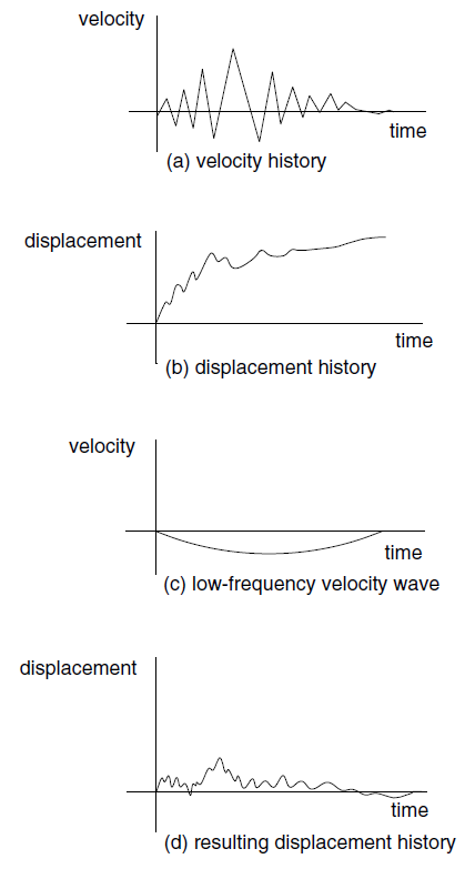
Figure 2: The baseline-correction process.
Quiet Boundaries
The modeling of geomechanics problems involves media which, at the scale of the analysis, are better represented as unbounded. Deep underground excavations are normally assumed to be surrounded by an infinite medium, while surface and near-surface structures are assumed to lie on a half-space. Numerical methods relying on the discretization of a finite region of space require that appropriate conditions be enforced at the artificial numerical boundaries. In static analyses, fixed or elastic boundaries (e.g., represented by boundary-element techniques) can be realistically placed at some distance from the region of interest. In dynamic problems, however, such boundary conditions cause the reflection of outward propagating waves back into the model, and do not allow the necessary energy radiation. The use of a larger model can minimize the problem, since material damping will absorb most of the energy in the waves reflected from distant boundaries. However, this solution leads to a large computational burden. The alternative is to use quiet (or absorbing) boundaries. Several formulations have been proposed. The viscous boundary developed by Lysmer and Kuhlemeyer (1969) is used in FLAC3D. It is based on the use of independent dashpots in the normal and shear directions at the model boundaries. The method is almost completely effective at absorbing body waves approaching the boundary at angles of incidence greater than 30°. For lower angles of incidence, or for surface waves, there is still energy absorption, but it is not perfect. However, the scheme has the advantage that it operates in the time domain. Its effectiveness has been demonstrated in both finite-element and finite-difference models (Kunar et al. 1977). A variation of the technique proposed by White et al. (1977) is also widely used.
More efficient energy absorption (particularly in the case of Rayleigh waves) requires the use of frequency-dependent elements, which can only be used in frequency-domain analyses (e.g., Lysmer and Waas 1972). These are usually termed “consistent boundaries” and involve the calculation of dynamic stiffness matrices coupling all the boundary degrees-of-freedom. Boundary-element methods may be used to derive these matrices (e.g., Wolf 1985). A comparative study of the performance of different types of elementary, viscous, and consistent boundaries was documented by Roesset and Ettouney (1977).
The quiet-boundary scheme proposed by Lysmer and Kuhlemeyer (1969) involves dashpots attached independently to the boundary in the normal and shear directions. The dashpots provide viscous normal and shear tractions given by
where \(v_n\) and \(v_s\), are the normal and shear components of the velocity at the boundary, \(\rho\) is the mass density, and \(C_p\) and \(C_s\) are the \(p\)- and \(s\)-wave velocities.
These viscous terms can be introduced directly into the equations of motion of the gridpoints lying on the boundary. A different approach, however, was implemented in FLAC3D, whereby the tractions \(t_n\) and \(t_s\) are calculated and applied at every timestep in the same way boundary loads are applied. This is more convenient than the former approach, and tests have shown that the implementation is equally effective. The only potential problem concerns numerical stability, because the viscous forces are calculated from velocities lagging by half a timestep. In practical analyses to date, no reduction of timestep has been required by the use of the nonreflecting boundaries. Timestep restrictions demanded by small zones are usually more important.
Dynamic analysis starts from some in-situ condition. If a fixed boundary is used while generating the static stress state, this boundary condition can be replaced by quiet boundaries; the boundary gridpoints will be freed, and the boundary reaction forces will be automatically calculated and maintained throughout the dynamic loading phase. However, changes in static loading during the dynamic phase should be avoided. For example, if a tunnel is excavated after quiet boundaries have been specified on the bottom boundary, the whole model will start to move upward. This is because the total gravity force no longer balances the total reaction force at the bottom that was calculated when the boundary was changed to a quiet one. If a stress boundary condition is used during the static solution, a stress boundary condition of opposite sign must also be applied over the same boundary when the quiet boundary is applied for the dynamic phase. This will allow the correct reaction forces to be in place at the boundary for the dynamic calculation.
Quiet boundary conditions can be applied in the global coordinate directions, or along
inclined boundaries, in the normal and shear directions using the zone face apply
command with appropriate keywords (quiet-normal, quiet-dip,
quiet-strike for one component or quiet for all three components). When using
the zone face apply command to install a quiet boundary condition, remember that the
material properties used in Equations (5) and (6) are obtained from
the zones immediately adjacent to the boundary. Thus, appropriate material properties for
boundary zones must be in place at the time the zone face apply command is given, in
order for the correct properties of the quiet boundary to be stored.
Quiet boundaries are best-suited when the dynamic source is within a grid. Quiet boundaries should not be used alongside boundaries of a grid when the dynamic source is applied as a boundary condition at the top or base, because the wave energy will “leak out” of the sides. In this situation, free-field boundaries (described below) should be applied to the sides.
Free-Field Boundaries
Numerical analysis of the seismic response of surface structures such as dams requires the discretization of a region of the material adjacent to the foundation. The seismic input is normally represented by plane waves propagating upward through the underlying material. The boundary conditions at the sides of the model must account for the free-field motion that would exist in the absence of the structure. In some cases, elementary lateral boundaries may be sufficient. For example, if only a shear wave were applied on the horizontal boundary, AC (shown in Figure 3), it would be possible to fix the boundary along AB and CD in the vertical direction only (see the example in Shear Wave Loading of a Model with Free-Field Boundaries). These boundaries should be placed at distances sufficient to minimize wave reflections and achieve free-field conditions. For soils with high material damping, this condition can be obtained with a relatively small distance (Seed et al. 1975). However, when the material damping is low, the required distance may lead to an impractical model. An alternative procedure is to “enforce” the free-field motion in such a way that boundaries retain their non-reflecting properties (i.e., outward waves originating from the structure are properly absorbed). This approach was used in the continuum finite-difference code NESSI (Cundall et al. 1980). A technique of this type involving the execution of free-field calculations in parallel with the main-grid analysis was developed for FLAC3D.
The lateral boundaries of the main grid are coupled to the free-field grid by viscous dashpots to simulate a quiet boundary (see Figure 3), and the unbalanced forces from the free-field grid are applied to the main-grid boundary. Both conditions are expressed in Equations (7), (8), and (9), which apply to the free-field boundary along one side-boundary plane with its normal in the direction of the \(x\)-axis. Similar expressions may be written for the other sides and corner boundaries:
where:
| \(\rho\) | = | density of material along vertical model boundary; |
| \(C_p\) | = | \(p\)-wave speed at the side boundary; |
| \(C_s\) | = | \(s\)-wave speed at the side boundary; |
| \(A\) | = | area of influence of free-field gridpoint; |
| \(v_x^m\) | = | \(x\)-velocity of gridpoint in main grid at side boundary; |
| \(v_y^m\) | = | \(y\)-velocity of gridpoint in main grid at side boundary; |
| \(v_z^m\) | = | \(z\)-velocity of gridpoint in main grid at side boundary; |
| \(v_x^{\rm ff}\) | = | \(x\)-velocity of gridpoint in side free field; |
| \(v_y^{\rm ff}\) | = | \(y\)-velocity of gridpoint in side free field; |
| \(v_z^{\rm ff}\) | = | \(z\)-velocity of gridpoint in side free field; |
| \(F_x^{\rm ff}\) | = | free-field gridpoint force with contributions from the \(\sigma_{xx}^{\rm ff}\) stresses of the free-field zones around the gridpoint; |
| \(F_y^{\rm ff}\) | = | free-field gridpoint force with contributions from the \(\sigma_{xy}^{\rm ff}\) stresses of the free-field zones around the gridpoint; and |
| \(F_z^{\rm ff}\) | = | free-field gridpoint force with contributions from the \(\sigma_{xz}^{\rm ff}\) stresses of the free-field zones around the gridpoint. |
In this way, plane waves propagating upward suffer no distortion at the boundary because the free-field grid supplies conditions that are identical to those in an infinite model. If the main grid is uniform, and there is no surface structure, the lateral dashpots are not exercised because the free-field grid executes the same motion as the main grid. However, if the main-grid motion differs from that of the free field (due to, say, a surface structure that radiates secondary waves), then the dashpots act to absorb energy in a manner similar to quiet boundaries.
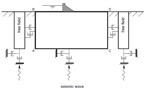
Figure 3: Model for seismic analysis of surface structures and free-field mesh.
In order to apply the free-field boundary in FLAC3D, the model must be oriented such that the base is horizontal and its normal is in the direction of the \(z\)-axis, and the sides are vertical and their normals are in the direction of either the \(x\)- or \(y\)-axis. If the direction of propagation of the incident seismic waves is not vertical, then the coordinate axes can be rotated such that the \(z\)-axis coincides with the direction of propagation. In this case, gravity will act at an angle to the \(z\)-axis, and a horizontal free surface will be inclined with respect to the model boundaries.
The free-field model consists of four plane free-field grids on the side boundaries of the model, and four column free-field grids at the corners (see Figure 4). The plane grids are generated to match the main-grid zones on the side boundaries, so that there is a one-to-one correspondence between gridpoints in the free field and the main grid. The four corner free-field columns act as free-field boundaries for the plane free-field grids. The plane free-field grids are two-dimensional calculations that assume infinite extension in the direction normal to the plane. The column free-field grids are one-dimensional calculations that assume infinite extension in both horizontal directions. Both the plane and column grids consist of standard FLAC3D zones, which have gridpoints constrained in such a way as to achieve the infinite extension assumption.
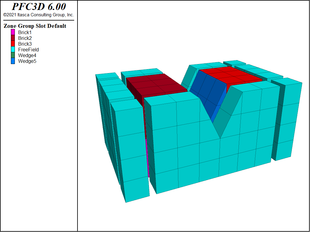
Figure 4: Side and corner free-field boundaries in a FLAC3D model.
The model should be in static equilibrium before the free-field boundary is applied.
The static equilibrium conditions prior to the dynamic analysis are transferred
to the free field automatically when the zone dynamic free-field command is invoked.
The free-field condition is applied to lateral boundary gridpoints.
All zone data (including model types and current state variables) in the model zones adjacent
to the free field are copied to the free-field region.
Free-field stresses are assigned the average stress of the neighboring grid zone.
The dynamic boundary conditions at the base of the model should be specified before applying the free-field.
These base conditions are automatically transferred to the free field when the free field is applied.
Note that the free field is continuous; if the main grid contains an interface that extends to a model boundary,
the interface will not continue into the free field.
After the zone dynamic free-field command is issued,
the free-field grid will plot automatically whenever the main grid is plotted.
Any model or nonlinear behavior may exist in the free field, as can fluid coupling and flow within the free field.
The following is a link to a simple example of the free-field boundary in use for the model shown in Figure 4.
Deconvolution and Selection of Dynamic Boundary Conditions
Design earthquake ground motions developed for seismic analyses are usually provided as outcrop motions, often rock outcrop motions. [1] However, for FLAC3D analyses, seismic input must be applied at the base of the model rather than at the ground surface, as illustrated in Figure 5. The question then arises: “What input motion should be applied at the base of a FLAC3D model in order to properly simulate the design motion?”
The appropriate input motion at depth can be computed through a “deconvolution” analysis using a 1D wave propagation code such as the equivalent-linear program SHAKE. This seemingly simple analysis is often the subject of considerable confusion resulting in improper ground motion input for FLAC3D models. The application of SHAKE for adapting design earthquake motions for FLAC3D input is described. Input of an earthquake motion into FLAC3D is typically done using one of the following:
- A rigid base, where an acceleration-time history is specified at the base of the FLAC3D mesh.
- A compliant base, where a quiet (absorbing) boundary is used at the base of the FLAC3D mesh.
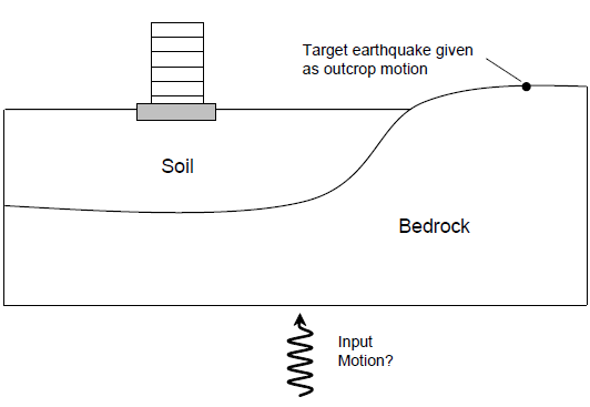
Figure 5: Seismic input to FLAC3D.
For a rigid base, a time history of acceleration (or velocity or displacement) is specified for gridpoints along the base of the mesh. While simple to use, a potential drawback of a rigid base is that the motion at the base of the model is completely prescribed. Hence, the base acts as if it were a fixed displacement boundary reflecting downward-propagating waves back into the model. Thus, a rigid base is not an appropriate boundary for general application unless a large dynamic impedance contrast is meant to be simulated at the base (e.g., low velocity sediments over high velocity bedrock).
For a compliant base simulation, a quiet boundary is specified along the base of the FLAC3D mesh. See the section on quiet boundaries. Note that if a history of acceleration is recorded at a gridpoint on the quiet base, it will not necessarily match the input history. The input stress-time history specifies the upward-propagating wave motion into the FLAC3D model, but the actual motion at the base will be the superposition of the upward motion and the downward motion reflected back from the FLAC3D model.
SHAKE (Schnabel et al. 1972) is a widely used 1D wave propagation code for site response analysis. SHAKE computes the vertical propagation of shear waves through a profile of horizontal visco-elastic layers. Within each layer, the solution to the wave equation can be expressed as the sum of an upward-propagating wave train and a downward-propagating wave train. The SHAKE solution is formulated in terms of these upward- and downward-propagating motions within each layer, as illustrated in Figure 6.
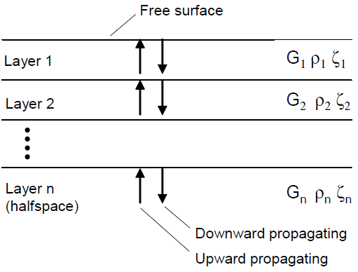
Figure 6: Layered system analyzed by SHAKE (layer properties are shear modulus, \(G\), density, \(\rho\) and damping fraction, \(\zeta\)).
The relation between waves in one layer and waves in an adjacent layer can be solved by enforcing the continuity of stresses and displacements at the interface between the layers. These well-known relations for reflected and transmitted waves at the interface between two elastic materials (Kolsky 1963) can be expressed in terms of recursion formulas. In this way, the upward- and downward-propagating motions in one layer can be computed from the upward and downward motions in a neighboring layer.
To satisfy the zero shear stress condition at the free surface, the upward- and downward-propagating motions in the top layer must be equal. Starting at the top layer, repeated use of the recursion formulas allows the determination of a transfer function between the motions in any two layers of the system. Thus, if the motion is specified at one layer in the system, the motion at any other layer can be computed.
SHAKE input and output is not in terms of the upward- and downward-propagating wave trains, but in terms of the motions at a) the boundary between two layers, referred to as a “within” motion, or b) at a free surface, referred to as an “outcrop” motion. The within motion is the superposition of the upward- and downward-propagating wave trains. The outcrop motion is the motion that would occur at a free surface at that location. Hence the outcrop motion is simply twice the upward-propagating wave-train motion. If needed, the upward-propagating motion can be computed by taking half the outcrop motion. At any point, the downward-propagating motion can then be computed by subtracting the upward-propagating motion from the within motion.
The SHAKE solution is in the frequency domain, with conversion to and from the time-domain performed with a Fourier transform. The deconvolution analysis discussed below illustrates the application of SHAKE for a linear, elastic case. See Comparison of FLAC3D to SHAKE for a Layered, Linear-Elastic Soil Deposit. SHAKE can also address nonlinear soil behavior approximately, through the equivalent linear approach. Analyses are run iteratively to obtain shear modulus and damping values for each layer that is compatible with the computed effective strain for the layer. See Comparison of FLAC3D to SHAKE for a Layered, Nonlinear-Elastic Soil.
Deconvolution for a Rigid Base — The deconvolution procedure for a rigid base is illustrated in Figure 7 for a two-dimensional FLAC simulation. The same procedure also applies to FLAC3D. The goal is to determine the appropriate base input motion to FLAC such that the target design motion is recovered at the top surface of the FLAC model. The profile modeled consists of three 20-m thick elastic layers with shear wave velocities and densities as shown in the figure. The SHAKE model includes the three elastic layers and an elastic half-space with the same properties as the bottom layer. The FLAC model consists of a column of linear elastic elements. The target earthquake is input at the top of the SHAKE column as an outcrop motion. Then, the motion at the top of the half-space is extracted as a within motion and is applied as an acceleration-time history to the base of the FLAC model. Mejia and Dawson (2006) show that the resulting acceleration at the surface of the FLAC model is virtually identical to the target motion. The SHAKE within motion is appropriate for rigid-base input because, as described above, the within motion is the actual motion at that location, the superposition of the upward- and downward-propagating waves.
Deconvolution for a Compliant Base — The deconvolution procedure for a compliant base is illustrated in Figure 8 for a FLAC simulation. Again, the same procedure applies to FLAC3D. The SHAKE and FLAC models are identical to those for the rigid body exercise, except that a quiet boundary is applied to the base of the FLAC mesh. For application through a quiet base, the upward-propagating wave motion (1/2 the outcrop motion) is extracted from SHAKE at the top of the half-space. This acceleration-time history is integrated to obtain a velocity, which is then converted to a stress history using Equation (4). Again, the resulting acceleration at the surface of the FLAC model is shown by Mejia and Dawson (2006) to be virtually identical to the target motion. As an additional check of the computed accelerations, they also show that the response spectra for both the compliant-base and rigid-base cases closely match the response spectra of the target motion.
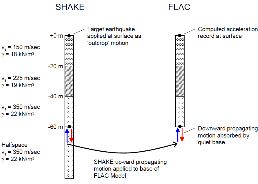
Figure 7: Deconvolution procedure for a rigid base (after Mejia and Dawson 2006).
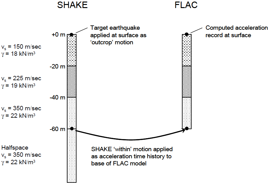
Figure 8: Deconvolution procedure for a compliant base (after Mejia and Dawson 2006).
Although useful for illustrating the basic ideas behind deconvolution, the previous example is not the typical case encountered in practice. The situation shown in Figure 9, where one or more soil layers (expected to behave nonlinearly) overlay bedrock (assumed to behave linearly), is more common. A FLAC or FLAC3D model for this case will usually include the soil layers and an elastic base of bedrock. To compute the correct FLAC3D compliant base input, a SHAKE model is constructed as shown in the figure. The SHAKE model includes a bedrock layer equal in thickness to the elastic base of the FLAC3D mesh, and an underlying elastic half-space with bedrock properties. The target motion is input to the SHAKE model as an outcrop motion at the top of the bedrock (point A). Designating this motion as outcrop means that the upward-propagating wave motion in the layer directly below point A will be set equal to 1/2 the target motion. The upward-propagating motion for input to FLAC3D is extracted at point B as 1/2 the outcrop motion.
For the compliant-base case, there is actually no need to include the soil layers in the SHAKE model, as these will have no effect on the upward-propagating wave train between points A and B. In fact, for this simple case, it is not really necessary to perform a formal deconvolution analysis, as the upward-propagating motion at point B will be almost identical to that at point A. Apart from an offset in time, the only differences will be due to material damping between the two points, which will generally be small for bedrock. Thus, for this very common situation, the correct input motion for FLAC3D is simply 1/2 of the target motion. (Note that the upward-propagating wave motion must be converted to a stress-time history using Equation (4), which includes a factor of 2 to account for the stress absorbed by the viscous dashpots.)
For a rigid-base analysis, the within motion at point B is required. Since this within motion incorporates downward-propagating waves reflected off the ground surface, the nonlinear soil layers must be included in the SHAKE model. However, soil nonlinearity will be modeled quite differently in FLAC3D and SHAKE. Thus, it is difficult to compute the appropriate FLAC3D input motion for a rigid-base analysis.
Another typical case encountered in practice is illustrated in Figure 10. Here, the soil profile is deep, and rather than extending the FLAC3D mesh all the way down to bedrock, the base of the model ends within the soil profile. Note that the mesh must be extended to a depth below which the soil response is essentially linear. Again, the design motion is input at the top of the bedrock (point A) as an outcrop motion, and the upward-propagating motion for input to FLAC3D is extracted at point B. As in the previous example, for a compliant-base analysis there is no need to include the soil layers above point B in the SHAKE model. These layers have no effect on the upward-propagating motion between points A and B. Unlike the previous case, the upward-propagating motion can be quite different at points A and B, depending on the impedance contrast between the bedrock and linear soil layer. Thus, it is not appropriate to skip the deconvolution analysis and use the target motion directly.
A rigid base is only appropriate for cases with a large impedance contrast at the base of the model. However, the use of SHAKE to compute the required input motion for a rigid base of a FLAC3D model leads to a good match between the target surface motion and the surface motion computed by FLAC3D only for a model that exhibits a low level of nonlinearity. The input motion already contains the effect of all layers above the base, because it contains the downward-propagating wave.
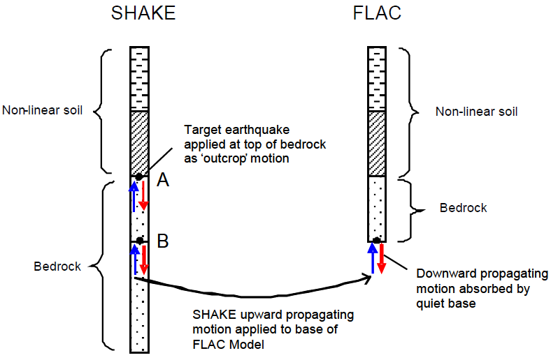
Figure 9: Compliant-base deconvolution procedure for a typical case (after Mejia and Dawson 2006).
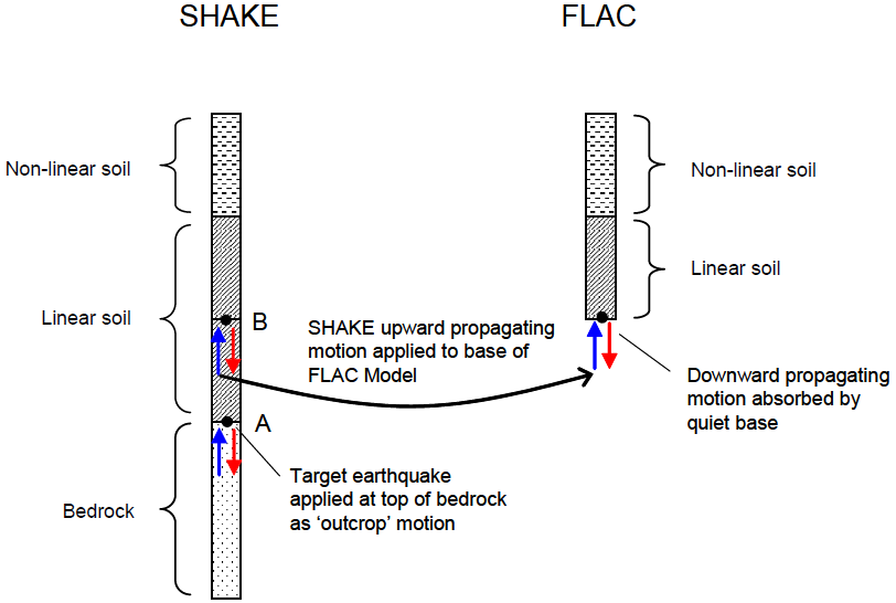
Figure 10: Compliant-base deconvolution procedure for another typical case (after Mejia and Dawson 2006).
A different approach must be taken if a FLAC3D model with a rigid base is used to simulate more realistic systems (e.g., sites that exhibit strong nonlinearity, or the effect of a surface or embedded structure). In the first case, the real nonlinear response is not accounted for by SHAKE in its estimate of base motion. In the second case, secondary waves from the structure will be reflected from the rigid base, causing artificial resonance effects.
A compliant base is almost always the preferred option because downward-propagating waves are absorbed. In this case, the quiet-base condition is selected, and only the upward-propagating wave from SHAKE is used to compute the input stress history. By using the upward-propagating wave only at a quiet FLAC3D base, no assumptions need to be made about secondary waves generated by internal nonlinearities or structures within the grid, because the incoming wave is unaffected by these; the outgoing wave is absorbed by the compliant base.
Although the presence of reflections from a rigid base is not always obvious in complex nonlinear FLAC3D analyses, they can have a major impact on analysis results, especially when cyclic-degradation or liquefaction-soil models are employed. Mejia and Dawson (2006) present examples from two-dimensional FLAC simulations that illustrate the nonphysical wave reflections calculated in models with a rigid base. One example, shown in Figure 11, demonstrates the difficulty with a rigid boundary. The nonphysical oscillations that result from a rigid base are shown by comparison to results for a compliant base in Figure 12. The inputs in both cases (rigid and compliant) were derived by deconvoluting the same surface motion.
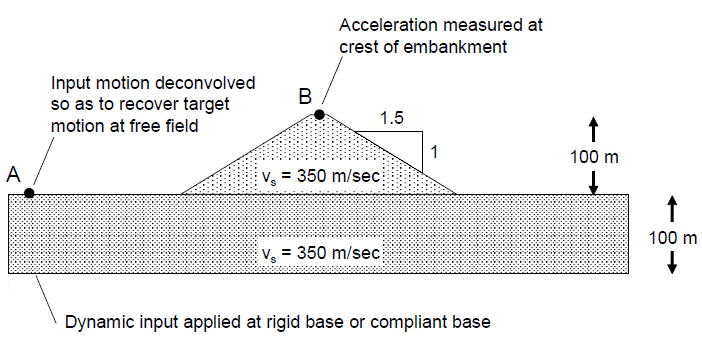
Figure 11: Embankment analyzed with a rigid and compliant base (after Mejia and Dawson 2006).
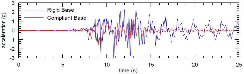
Figure 12: Computed accelerations at crest of embankment (after Mejia and Dawson 2006).
Hydrodynamic Pressures
The dynamic interaction between water in a reservoir and a concrete dam can have a significant influence on the performance of the dam during an earthquake. Westergaard (1933) established a mathematical basis for procedures to represent this interaction, and this approach is commonly used in engineering practice. Although the advent of computers has enabled numerical solution of coupled differential equations of fluid-structure systems, the formula proposed by Westergaard is widely used for stability analysis of smaller dams and preliminary calculations in the design of large dams.
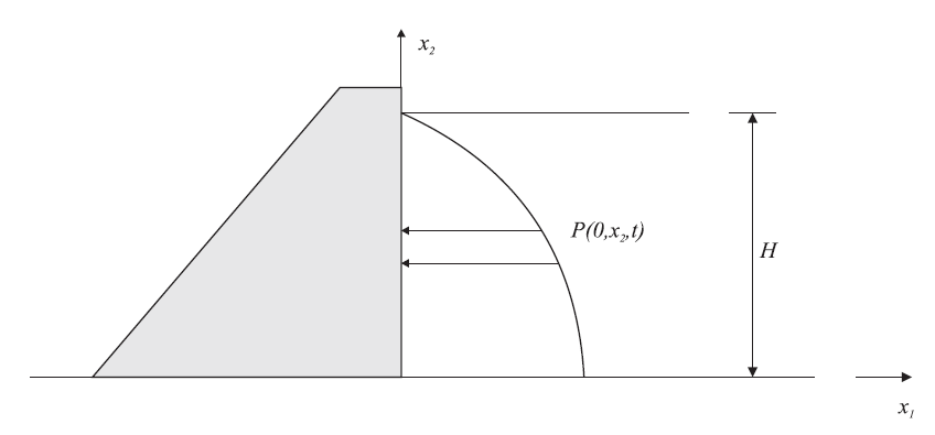
Figure 13: Hydrodynamic pressure acting on a rigid dam with a vertical upstream face.
The hydrodynamic pressure acting on a rigid concrete dam over a reservoir height, \(H\), is depicted in Figure 13. The pressure can be derived from the equation of motion for a fluid. The equation of motion for a fluid with small Reynold’s number can be written as
where \(c\) is the speed of sound in water and \(\Phi\) is the velocity potential. The water pressure can be written as a function of the velocity potential:
where \(\rho_w\) is the density of water.
Additional assumptions are made to simplify the loading condition:
- The water is assumed to be incompressible, which reduces Equation (10) to the Laplace equation: \(\frac{\delta^2 \Phi}{\delta x_1^2} + \frac{\delta^2 \Phi}{\delta x_2^2} = 0\).
- The free surface of the reservoir is assumed to be at rest. Thus, \(\frac{\delta \Phi}{\delta t} = 0\) at \(x_2 = H\).
- The reservoir is assumed to be infinitely long. Therefore, as \(x_1 \rightarrow \infty, \Phi \rightarrow 0\).
- Hydrodynamic motion is assumed to be horizontal only: \(\frac{\delta \Phi}{x_2} = 0\) at \(x_2 = 0\).
- The upstream face of the dam is vertical and the dam is rigid: \(\frac{\delta \Phi}{x_1} = f(t)\) at \(x_1 = 0\).
The solution of Equation (10) with the preceding assumptions can be obtained for an arbitrary acceleration, \(\ddot{x}_0 (t)\), in the form of an infinite Fourier series:
Equation (11) can be approximated as
where \(C_m\) = 0.743 and \(\ddot{x}\) is the horizontal acceleration at the dam face.
Equation (12) is implemented in FLAC3D by adjusting the grid point mass on the upstream face of the dam to account for the hydrodynamic pressure. The equivalent pressure, \(\bar{p}\), resulting from the inertial forces associated with the gridpoint and the hydrodynamic pressure of the water in the reservoir, averaged over the area associated with the gridpoint, can be written as
where \(A_g\) is the area associated with the gridpoint, \(\Delta x_2\) is the contact length on the upstream face of the dam through which the water load is applied for the gridpoint, and \(\rho_ec\) is the equivalent density of the gridpoint and is given by
where
\(\rho_c\) is the density of concrete such that the gridpoint mass is given by \(m_g = A_g \rho_c\). The scaled gridpoint mass, \(m_sg = A_g \rho_ec\), is used only for the motion calculation in the horizontal direction; the effect of the increase mass does not influence the vertical forces.
The gridpoint mass is adjusted by adding the term (as determined by Equation
(13)) to account for the hydrodynamic pressure. This adjustment is stored in
a location that is modifiable using the FISH gridpoint function gp.mass.add.
The conditions are applied using the zone face westergaard command.
The following simple example is provided that illustrates the effect of hydrodynamic pressures and compares the Westergaard approximation to the result of explicitly modeling the water using FLAC3D zones.
Wave Transmission
Accurate Wave Propagation
Numerical distortion of the propagating wave can occur in a dynamic analysis as a function of the modeling conditions. Both the frequency content of the input wave and the wave speed characteristics of the system will affect the numerical accuracy of wave transmission. Kuhlemeyer and Lysmer (1973) show that, for accurate representation of wave transmission through a model, the spatial element size, \(\Delta l\), must be smaller than approximately one-tenth to one-eighth of the wavelength associated with the highest frequency component of the input wave. For instance,
where \(\lambda\) is the wavelength associated with the highest frequency component that contains appreciable energy.
Filtering
For dynamic input with a high peak velocity and short rise time, the Kuhlemeyer and Lysmer requirement may necessitate a very fine spatial mesh and a corresponding small timestep. The consequence is that reasonable analyses may be prohibitively time- and memory-consuming. In such cases, it may be possible to adjust the input by recognizing that most of the power for the input history is contained in lower-frequency components (e.g., use “fft.fis” in “datafiles\FISH\Library”). By filtering the history and removing high frequency components, a coarser mesh may be used without significantly affecting the results.
The filtering procedure can be accomplished with a low-pass filter routine such as the fast Fourier transform technique. For example, the unfiltered velocity record shown in Figure 14 represents a typical waveform containing a very high frequency spike. The highest frequency of this input exceeds 50 Hz but, as shown by the power spectral density plot of Fourier amplitude versus frequency (Figure 15), most of the power (approximately 99%) is made up of components of frequency 15 Hz or lower. It can be inferred, therefore, that by filtering this velocity history with a 15 Hz low-pass filter, less than 1% of the power is lost. The input filtered at 15 Hz is shown in Figure 16, and the Fourier amplitudes are plotted in Figure 17. The difference in power between unfiltered and filtered input is less than 1%, while the peak velocity is reduced 38%, and the rise time is shifted from 0.035 to 0.09 seconds. Analyses should be performed with input at different levels of filtering to evaluate the influence of the filter on model results.
If a simulation is run with an input history that violates Equation (14), the output will contain spurious “ringing” (superimposed oscillations) that are nonphysical. The input spectrum must be filtered before being applied to a FLAC3D grid. This limitation applies to all numerical models in which a continuum is discretized; it is not just a characteristic of FLAC3D. Any discretized medium has an upper limit to the frequencies that it can transmit, and this limit must be respected for the results to be meaningful. Users of time-domain codes commonly apply sharp pulses or step waveforms to the numerical grid; this is not acceptable, since these waveforms have spectra that extend to infinity. It is a simple matter to apply, instead, a smooth pulse that has a limited spectrum. Alternatively, artificial viscosity may be used to spread sharp wave-fronts over several zones (see Artificial Viscosity), but this method strictly only applies to isotropic strain components.
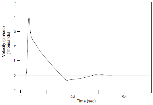
Figure 14: Unfiltered velocity history.
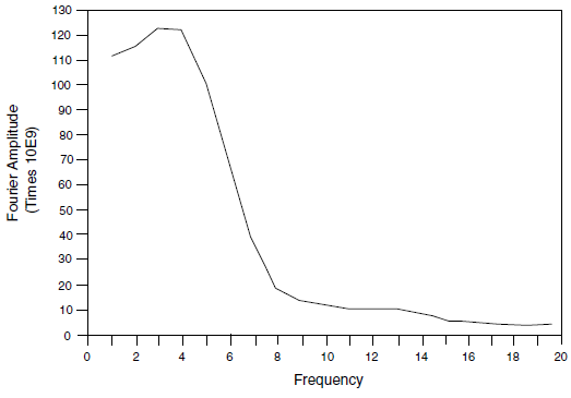
Figure 15: Unfiltered power spectral density plot.
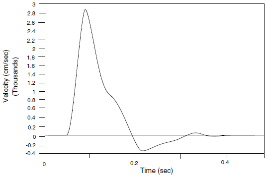
Figure 16: Filtered velocity history at 15 Hz.
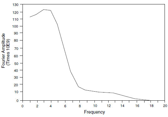
Figure 17: Results of filtering at 15 Hz.
Mechanical Damping and Material Response
Natural dynamic systems contain some degree of damping of the vibration energy within the system; otherwise, the system would oscillate indefinitely when subjected to driving forces. Damping is due, in part, to energy loss as a result of internal friction in the intact material and slippage along interfaces, if these are present.
FLAC3D uses a dynamic algorithm for solution of two general classes of mechanical problems: quasi-static and dynamic. Damping is used in the solution of both classes of problems, but quasi-static problems require more damping for rapid convergence to equilibrium. The damping for static solutions is discussed in Mechanical Damping.
For a dynamic analysis, the damping in the numerical simulation should reproduce, in magnitude and form, the energy losses in the natural system when subjected to a dynamic loading. In soil and rock, natural damping is mainly hysteretic (i.e., independent of frequency—see Gemant and Jackson 1937, and Wegel and Walther 1935). It is difficult to reproduce this type of damping numerically because of at least two problems (see Cundall 1976, and comments in Characteristics of Fully Nonlinear Method). First, many simple hysteretic functions do not damp all components equally when several waveforms are superimposed. Second, hysteretic functions lead to path-dependence, which makes results difficult to interpret. However, if a constitutive model that contains an adequate representation of the hysteresis that occurs in a real material is found, then no additional damping would be necessary. This comment is addressed to users who program their own constitutive models in C++; the built-in models are not considered to model dynamic hysteresis well enough to omit additional damping completely.
For several reasons, it is impractical to use the “real” stress/strain response of the material in numerical simulations. For example: 1) there are no laws that describe the complete material response; and 2) existing laws that capture many important aspects have many material parameters requiring extensive calibration.
In time-domain programs, Rayleigh damping is commonly used to provide damping that is approximately frequency-independent over a restricted range of frequencies. Although Rayleigh damping embodies two viscous elements (in which the absorbed energy is dependent on frequency), the frequency-dependent effects are arranged to cancel out at the frequencies of interest.
Hysteretic damping is an alternative damping option. This form of damping allows strain-dependent modulus and damping functions to be incorporated directly into the FLAC3D simulation. This makes it possible to make direct comparisons between calculations made with the equivalent-linear method and a fully nonlinear method, without making any compromises in the choice of constitutive model.
For routine engineering design, we must use an approximate representation of cyclic energy dissipation. In FLAC3D, when using simple plasticity models such as Mohr-Coulomb, the choice is between Rayleigh damping and hysteretic damping. Here, we make some general comparisons between the two approaches, enabling a choice to be made. In general, hysteretic damping is the more realistic of the two, and it entails no reduction in timestep. For further discussion, see Integration of Damping Schemes and Nonlinear Material Models for Geo-materials.
For low levels of cyclic strain and fairly uniform conditions, Rayleigh damping and hysteretic damping give similar results, provided that the levels of damping set for both are consistent with the levels of cyclic strain experienced. The results will differ in the following two circumstances:
1. When the system is nonuniform (e.g., layers of quite different properties), then cyclic strain levels may be different in different locations and at different times. Using hysteretic damping, these different strain levels produce realistically different damping levels in time and space, while constant and uniform Rayleigh damping parameters can only reproduce the average response. It would be possible to adjust the Rayleigh damping parameters to account for spatial variations in damping using an iterative (strain-compatible) scheme, as used in the equivalent-linear method. It may also be possible to adjust the Rayleigh damping parameters in time, although some practical difficulties may be encountered.
2. As yield is approached, neither Rayleigh damping nor hysteretic damping account for the energy dissipation of extensive yielding. Thus, irreversible strain occurs externally to both schemes, and dissipation is represented by the yield model (e.g., Mohr-Coulomb). Under this condition, the mass-proportional term of Rayleigh damping may inhibit yielding because rigid-body motions that occur during failure modes are erroneously resisted. Hysteretic damping may give rise to larger permanent strains in such a situation, but this condition is usually believed to be more realistic compared to one using Rayleigh damping.
We note that hysteretic damping provides almost no energy dissipation at very low cyclic strain levels, which may be unrealistic. To avoid low-level oscillation, it is recommended that a small amount (e.g., 0.2%) of stiffness-proportional Rayleigh damping be added when hysteretic damping is used in a dynamic simulation.
Another form of damping in FLAC3D, the local damping embodied in FLAC3D’s static solution scheme, may be used dynamically, but with a damping coefficient appropriate to wave propagation. Local damping in dynamic problems is useful as an approximate way to include hysteretic damping. However, it becomes increasingly unrealistic as the complexity of the waveforms increases (i.e., as the number of frequency components increases). Local damping cannot properly capture the energy loss of multiple frequency cyclic loading.
A fourth form of damping, artificial viscosity, is also provided in FLAC3D. This damping may be used for analyses involving sharp dynamic fronts.
Rayleigh Damping
Rayleigh damping was originally used in the analysis of structures and elastic continua to damp the natural oscillation modes of the system. The equations, therefore, are expressed in matrix form.
A damping matrix, \(C\), is used with components proportional to the mass, \(M\), and stiffness, \(K\), matrices:
where \(\alpha\) is the mass-proportional damping constant; and \(\beta\) is the stiffness-proportional damping constant.
The mass-proportional term is analogous to a dashpot connecting every FLAC3D gridpoint to “ground.” The stiffness-proportional term is analogous to a dashpot connected across each FLAC3D zone (responding to the strain rate). Although both terms are frequency-dependent, an approximately frequency-independent response can be obtained over a limited frequency range with the appropriate choice of parameters as discussed below.
For a multiple degree-of-freedom system, the critical damping ratio, \(\xi_i\), at any angular frequency of the system, \(\omega_i\), can be found from (Bathe and Wilson 1976)
or
The critical damping ratio, \(\xi_i\), is also known as the fraction of critical damping for mode \(i\) with angular frequency \(\omega_i\).
Figure 18 shows the variation of the normalized critical damping ratio with angular frequency \(\omega_i\). Three curves are given: mass components only; stiffness components only; and the sum of both components. As shown, mass-proportional damping is dominant at lower angular-frequency ranges, while stiffness-proportional damping dominates at higher angular frequencies. The curve representing the sum of both components reaches a minimum at
or
The center frequency is then defined as
Note that at frequency \(\omega_{\min}\) (or \(f_{\min}\)) (and only at that frequency), mass damping, and stiffness damping each supply half of the total damping force.
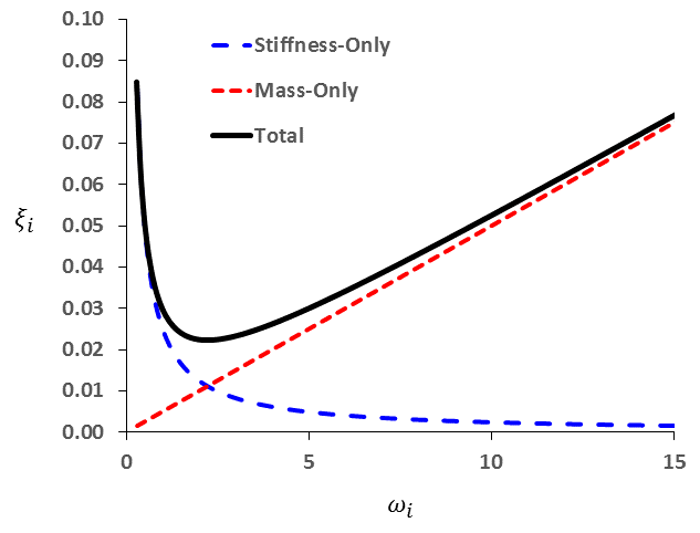
Figure 18: Variation of normalized critical damping ratio with angular frequency.
Rayleigh damping is specified in FLAC3D with the parameters \(f_{\min}\)
in Hertz (cycles per second) and \(\xi_{\min}\), both specified with the
zone dynamic damping rayleigh command.
Stiffness-proportional damping causes a reduction in the critical timestep for the explicit solution scheme (see Belytschko 1983). As the damping ratio corresponding to the highest natural frequency is increased, the timestep is reduced (see Dynamic Timestep). This can result in a substantial increase in runtimes for dynamic simulations.
In FLAC3D, the internal timestep calculation takes account of stiffness-proportional
damping, but it is still possible for instability to occur if the large-strain calculation
is in effect (model largestrain) and very large mesh deformation occurs.
If this happens, it is necessary to reduce the timestep manually (via the
model dynamic timestep fix command).
For the case shown in Figure 18, \(\omega_{\min} = 10\) radians per second. It is evident that the damping ratio is almost constant over at least a 3:1 frequency range (e.g., from 5 to 15). Since damping in geologic media is commonly independent of frequency (as discussed in Dynamic Mechanical Damping), \(\omega_{\min}\) is usually chosen to lie in the center of the range of frequencies present in the numerical simulation — either natural frequencies of the model or predominant input frequencies. Hysteretic damping is thereby simulated in an approximate fashion.
Viscous stress increments representing the stiffness-proportional component of Rayleigh damping are added to the total stress increments during a timestep in order to compute gridpoint forces. Thus,
where \(\sigma_v\) is a component of the combined stress tensor used to derive gridpoint forces, \(\sigma_n\) is the corresponding component returned from the constitutive law, and \(\sigma_o\) is the value of the component prior to invoking the constitutive law. The notation \(\bigl\{\) \(\bigr\}\) denotes the vector of all components.
Viscous stresses are not included with the accumulated total stresses (\(\sigma_n\)).
A stiffness matrix is not needed in this formulation. Rayleigh damping operates directly on the tangent modulus for the constitutive model, whether it is linear or nonlinear.
Stiffness-proportional damping is turned off when plastic failure occurs within a FLAC3D
zone. Mass-proportional damping, however, remains active. If excessive failure occurs in a
model, the mass-proportional term may inhibit yielding. In this case, it may be advisable to
exclude Rayleigh damping from regions of strong plastic flow (by using the
zone dynamic damping rayleigh command to set Rayleigh damping in selected regions,
as described in Spatial Variation in Damping).
Example Application of Rayleigh Damping
In order to demonstrate how Rayleigh damping works in FLAC3D, the following simple example examines the results of four damping cases for comparison.
Guidelines for Selecting Rayleigh Damping Parameters
Damping Ratio, \(\xi_{\min}\)
What is normally attempted in a dynamic analysis is the reproduction of the frequency-independent damping of materials at the correct level. For geological materials, damping commonly falls in the range of 2 to 5% of critical; for structural systems, 2 to 10% is representative (Biggs 1964). Also, see Newmark and Hall (1982) for recommended damping values for different materials. In analyses that use one of the plasticity constitutive models (e.g., Mohr-Coulomb), a considerable amount of energy dissipation can occur during plastic flow. Thus, for many dynamic analyses that involve large-strain, only a minimal percentage of damping (e.g., 0.5%) may be required. Further, dissipation will increase with amplitude for stress/strain cycles that involve plastic flow. \(\xi_{\min}\) is adjusted to coincide with the correct physical damping ratio.
The equivalent-linear program SHAKE (Schnabel, Lysmer, and Seed 1972) can be used to estimate material damping to represent the inelastic cyclic behavior of soils. An equivalent-linear analysis is performed for a layered soil deposit using the shear wave speeds and densities for the different layers. Strain-compatible values for the damping ratios and shear-modulus reduction factors are then determined. Average damping ratios and shear modulus reduction factors are estimated for each layer; the damping ratios are the estimates for input in the Rayleigh damping in FLAC3D.
Center Frequency, \(f_{\min}\)
Rayleigh damping is frequency-dependent but has a “flat” region that spans about a 3:1 frequency range, as shown in Figure 18. For any particular problem, a spectral analysis of typical velocity records might produce a response such as the one shown in Figure 19. [2]
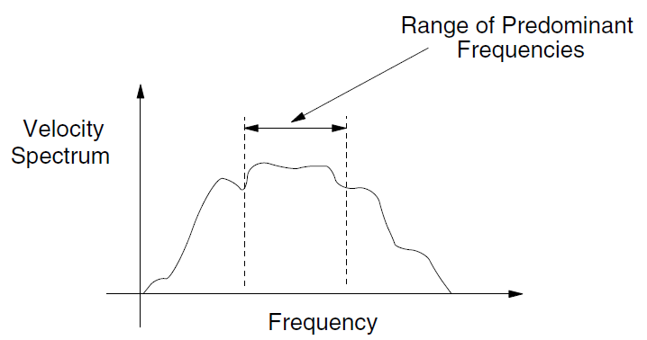
Figure 19: Plot of velocity spectrum versus frequency.
If the highest predominant frequency is three times greater than the lowest predominant frequency, then there is a 3:1 span or range that contains most of the dynamic energy in the spectrum. The idea in dynamic analysis is to adjust \(f_{\min}\) of the Rayleigh damping so that its 3:1 range coincides with the range of predominant frequencies in the problem. The predominant frequencies are neither the input frequencies nor the natural modes of the system, but a combination of both. The idea is to try to get the right damping for the important frequencies in the problem.
For many problems, the important frequencies are related to the natural mode of oscillation of the system. Examples of this type of problem include seismic analysis of surface structures such as dams, or dynamic analysis of underground excavations. The fundamental frequency, \(f\), associated with the natural mode of oscillation of a system is
where \(C\) is the speed of propagation associated with the mode of oscillation, and \(\lambda\) is the longest wavelength associated with the mode of oscillation.
For a continuous, elastic system (e.g., a one-dimensional elastic bar), the speed of propagation, \(C_p\), for \(p\)-waves is given by Equation (3), and for \(s\)-waves by Equation (4). If shear motion of the bar gives rise to the lowest natural mode, then \(C_s\) is used in the above equation; otherwise, \(C_p\) is used if motion parallel to the axis of the bar gives rise to the lowest natural mode.
The longest wavelength (or characteristic length or fundamental wavelength) depends on boundary conditions. Consider a solid bar of unit length with boundary conditions as shown in Figure 20a. The fundamental mode shapes for cases (1), (2), and (3) are as shown in Figure 20b. If a wavelength for the fundamental mode of a particular system cannot be estimated in this way, then a preliminary run may be made with zero damping (for example, see Mechanical Damping). A representative natural period may be estimated from time histories of velocity or displacement. Natural Periods of an Elastic Column contains a simple example in which natural periods are estimated by undamped simulations.
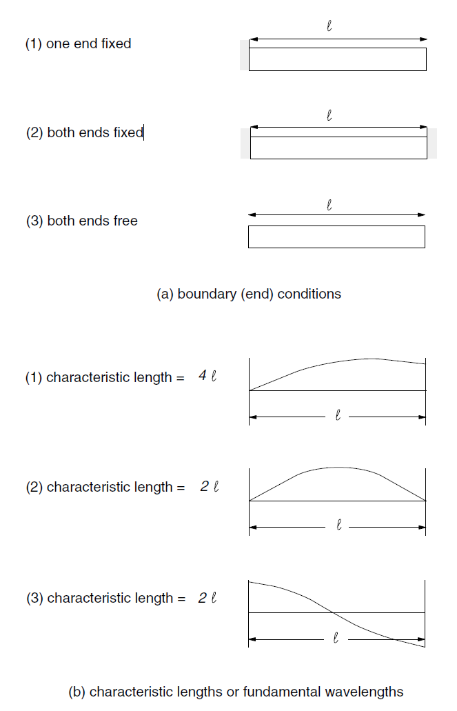
Figure 20: Comparison of fundamental wavelengths for bars with varying end conditions.
Hysteretic Damping
The equivalent-linear method has been in use for many years to calculate the wave propagation (and response spectra) in soil and rock at sites subjected to seismic excitation. The method does not directly capture any nonlinear effects because it assumes linearity during the solution process; strain-dependent modulus and damping functions are only taken into account in an average sense in order to approximate some effects of nonlinearity (damping and material softening). Although fully nonlinear codes such as FLAC3D are capable—in principle—of modeling the correct physics, it has been difficult to convince designers and licensing authorities to accept fully nonlinear simulations. One reason is that the constitutive models available to FLAC3D are either too simple (e.g., an elastic/plastic model, which does not reproduce the continuous yielding seen in soils), or too complicated (e.g., the Wang model [Wang et al. 2001], which needs many parameters and a lengthy calibration process). Further, there is a need to directly accept the same degradation curves used by equivalent-linear methods (see Figure 21 and 22 for examples), to allow engineers to move easily from using these methods to using fully nonlinear methods.
A further motivation for incorporating such cyclic data into a hysteretic damping model for FLAC3D is that the need for additional damping such as Rayleigh damping would be eliminated. Rayleigh damping is unpopular with code users because it often involves a drastic reduction in timestep, and a consequent increase in solution time.
Optional hysteretic damping is described here; it may be used on its own or in conjunction with the other damping schemes, such as Rayleigh damping or local damping. (It may also be used with some of the built-in constitutive models except for the models with nonlinear elastic moduli, e.g., modified Cam-Clay.)
The hysteretic damping formulation is not intended to be a complete constitutive model: it should be used as a supplement to one of the built-in nonlinear models, and not as a primary way to simulate yielding. If models that embody both plastic yield and an adequate hysteretic response are used, then there is no reason to add further damping; the hysteretic damping option in FLAC3D is only intended to provide damping for those models lacking intrinsic damping when not yielding. Further, Rayleigh damping should be unnecessary when hysteretic damping is in operation, apart from its possible use (at low levels: e.g., 0.2%) to remove high frequency noise.
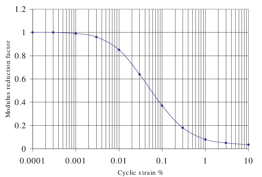
Figure 21: Modulus reduction curve for sand (Seed & Idriss 1970 — “upper range”). The data set is from the file supplied with the SHAKE-91 code download. (https://nisee.berkeley.edu/elibrary/getpkg?id=SHAKE91)
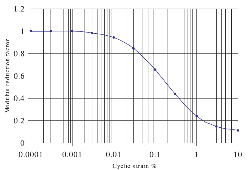
Figure 22: Modulus reduction curve for clay (Sun et al. 1988 — “upper range”). The data set is from the file supplied with the SHAKE-91 code download. (https://nisee.berkeley.edu/elibrary/getpkg?id=SHAKE91)
Hysteretic Damping Formulation, Implementation, and Calibration
Formulation
Modulus degradation curves, as illustrated in Figures 21 and 22, imply a nonlinear stress/strain curve. If we assume an ideal soil, in which the stress depends only on the strain (not on the number of cycles, or time), we can derive an incremental constitutive relation from the degradation curve, described by \(\bar {\tau} / \gamma = M_s\), where \(\bar {\tau}\) is the normalized shear stress, \(\gamma\) is the shear strain, and \(M_s\) is the normalized secant modulus.
where \(M_t\) is the normalized tangent modulus. The incremental shear modulus in a nonlinear simulation is then given by \(G_o M_t\). This is used in place of the given shear modulus, \(G_o\) (i.e., the property assigned with the name shear).
In order to handle two- and three-dimensional strain paths, an approach similar to the one described for the Finn model (see Simple Model Formulations) is used, whereby the shear strain is decomposed into components in strain space, and strain reversals are detected by changes in signs of the dot product of the current increment and the previous mean path. Following the formulation of the Finn model (replacing \(\epsilon\) with \(\gamma\) but otherwise using the same notation):
A reversal is detected when \(|d|\) passes through a maximum, and the previous-reversal strain values are updated as given by Equations (37) and (38). Note that there is no “latency” period, as used in the Finn model (see Simple Model Formulations); there is no minimum number of timesteps that must occur before a reversal is detected.
Between reversals, the shear modulus is multiplied by \(M_t\), using \(\gamma = |d|\) in Equation (26). The multiplier is applied to the shear modulus used in all built-in constitutive models, except for the transversely isotropic elastic, modified Cam-clay, and creep material models.
Implementation
The formulation described above is implemented in FLAC3D, by modifying the strain-rate calculation so that the mean strain-rate tensor (averaged over all subzones) is calculated before any calls are made to constitutive model functions. At this stage, the hysteretic logic is invoked, returning a modulus multiplier, which is passed to any called constitutive model. The model then uses the multiplier \(M_t\) to adjust the apparent value of tangent shear modulus of the full zone being processed.
In addition to the “backbone curve,’’ provided by applying Equation (26) to a modulus degradation curve (described below), two Masing (1926) rules are used to specify the behavior at reversal points. Essentially, these state that: 1) a new (but inverted) function is started upon reversal, implying that the initial unload modulus is \(G\); and 2) the first quarter-cycle of loading is scaled by one-half relative to all other cycles. Although Pyke (2004) concludes that “neither of the Masing rules is valid,” some simplifying assumption is necessary to ensure repeatable, closed loops. The fact that real soil departs from this ideal behavior is not believed to be too important in this context because the formulation is not intended to be a complete constitutive model, but simply to provide hysteretic damping as an alternative to Rayleigh damping.
An additional rule deals with sub-cycles: the hysteretic logic contains push-down FILO (first in, last out) stacks that record all state information (e.g., stress, strain, tangent modulus, and previous reversal point) at the point of reversal, for both positive—and negative—going strain directions. If the strain level returns to—and exceeds—a previous value recorded in the stack (of the appropriate sign), the state information is popped from the stack, so that the behavior (and, hence, tangent multiplier) reverts back to that which was applied at the time before the reversal.
The operation of these various rules in illustrated in the following simple example:
The degradation curves used in earthquake engineering are usually given as tables of values, with cyclic strains spaced logarithmically. Since the derivative of the modulus-reduction curve is required here (i.e., for Equation (26)), the coarse spacing (e.g., 11 points in the curve shown in Figure 22) leads to unacceptable errors if numerical derivatives are calculated. Thus, the implemented hysteretic model uses only continuous functions to represent the modulus-reduction curve, so that analytical derivatives may be calculated. The various implemented functions are described in the following section. If degradation curves are available only in table form, they must be fitted to one of the built-in functional forms before simulations can be performed.
The hysteretic damping feature is invoked with the command
zone dynamic damping hysteretic name <v1 v2 v3 …> <range>
where name is the name of the fitting function (chosen from default, sig3, sig4, and hardin — see the following discussion), and v1, v2, v3, …, are numerical values for function parameters. The optional range may be any acceptable range phrase for zones.
Hysteretic damping may be removed from any range of zones with the command
zone dynamic damping hysteretic off <range>
Note that the zone dynamic damping hysteretic command only applies where the
model configure dynamic mode of operation has been selected and when
model configure dynamic applies. Hysteretic damping operates independent of all other
forms of damping, which may be also specified to operate “in parallel” with hysteretic
damping.
Tangent-Modulus Functions
Various built-in functions are available to represent the variation of the shear modulus
reduction factor, \(G/G_{\rm max}\), with cyclic strain (given in percent),
according to the keyword specified on the zone dynamic damping hysteretic command.
Default model — default
The default hysteresis model is developed by noting that the S-shaped curve of modulus versus logarithm of cyclic strain can be represented by a cubic equation, with zero slope at both low strain and high strain. Thus, the secant modulus \(M_s\) is
where
and \(L\) is the logarithmic strain,
The parameters \(L_1\) and \(L_2\) are the extreme values of logarithmic strain (i.e., the values at which the tangent slope becomes zero). Thus, giving \(L_1 = -3\) and \(L_2 = 1\) means that the S-shaped curve will extend from a lower cyclic strain of 0.001% (10-3) to an upper cyclic strain of 10% (101). Since the slopes are zero at these limits, it is not meaningful to operate the damping model with strains outside the limits. (Note that Equation (39) is only assumed to apply for \(0 \leq s \leq 1\), and that the tangent modulus will be set to zero otherwise.) The tangent modulus is given by
Using the chain rule,
we obtain
There is a further limit, \(s > s_{\rm min}\), such that the tangent modulus is always positive (no strain softening). Thus,
or
where \(A = 6 {\rm log}_{10}e / (L_2 - L_1)\). The lowest positive root is
In applying the model, \(M_t = 0$ if $s < s_{\rm min}\).
The default model function can be fit to degradation curves by using a curve-fitting graphing software (e.g., SigmaPlot, http://www.systat.com/products/sigmaplot/ ). For example, the numerical best-fit of the default model to the curves of Figures 21 and 22 are listed in Tables 3 and 4, respectively.
Sigmoidal models — sig3, sig4
Sigmoidal curves are monotonic within the defined range and have the appropriate asymptotic behavior. Thus the functions are well-suited to represent modulus degradation curves. The two types of sigmoidal model (3 and 4 parameters, respectively) are
sig3 model
sig4 model
The command line for invoking these models requires that three symbols, \(a\), \(b\), and \(x_o\), are defined by the parameters v1, v2, and v3, respectively, for model sig3 (Equation (48)). For model sig4 (Equation (49)), the four symbols, \(a\), \(b\), \(x_o\), and \(y_o\), are entered by means of the parameters v1, v2, v3, and v4, respectively. Numerical fits for the two models to the curves of Figures 21 and 22 are provided in Tables 3 and 4, respectively.
Hardin/Drnevich model — hardin
The following function was suggested by Hardin and Drnevich (1972):
It has the useful property that the modulus reduction factor is 0.5 when \(\gamma = \gamma_{\rm ref}\), so that the sole parameter, \(\gamma_{\rm ref}\), may be determined (by inspection) from the strain at which the modulus-reduction curve crosses the \(G / G_{\rm max}\) = 0.5 line. Choosing a value of \(\gamma_{\rm ref}\) = 0.06 produces a match to the curve of Figure 21, and a value of 0.234 produces a match to the curve of Figure 22.
| Data set | Default | Sig3 | Sig4 | Hardin |
|---|---|---|---|---|
| Sand–upper range | \(L_1\) = -3.325 | \(a\) = 1.014 | \(a\) = 0.9762 | \(\gamma_{\rm ref}\) = 0.060 |
| (Seed &Idriss 1970) | \(L_2\) = 0.823 | \(b\) = -0.4792 | \(b\) = -0.4393 | |
| \(x_o\) = -1.249 | \(x_o\) = -1.285 | |||
| \(y_o\) = 0.03154 |
| Data set | Default | Sig3 | Sig4 | Hardin |
|---|---|---|---|---|
| Clay–upper range | \(L_1\) = -3.156 | \(a\) = 1.017 | \(a\) = 0.922 | \(\gamma_{\rm ref}\) = 0.234 |
| (Sun at el. 1988) | \(L_2\) = 1.904 | \(b\) = -0.5870 | \(b\) = -0.481 | |
| \(x_o\) = -0.633 | \(x_o\) = -0.745 | |||
| \(y_o\) = 0.0823 |
Calibration of Degradation Curves
Calibration of the tangent-modulus function involves both a comparison of the function results to the target shear-modulus reduction curve and a comparison to the target damping-ratio curve. The following simple example is provided for illustration and discussion:
In most attempts to match laboratory and numerical damping curves, it is noted that the damping provided by the hysteretic formulation at low cyclic strain levels is lower than that observed in the laboratory. This may lead to low-level noise, particularly at high frequencies. Although such noise hardly affects the essential response of the systems, for cosmetic reasons it may be removed by adding a small amount of Rayleigh damping. It is found that 0.2% Rayleigh damping (at an appropriate center frequency) is usually sufficient to remove residual oscillations without affecting the solution timestep.
Simple Application
The example provided below models a 20 m layer excited by a digitized earthquake to show that plausible behavior occurs for a case involving wave propagation, multiple and nested loops, and reasonably large cyclic strain.
Observations
A method has been developed to use cyclic modulus-degradation data directly in a FLAC3D simulation. The resulting model is able to reproduce the results of constant-amplitude cyclic tests, but it is also able to accommodate strain paths that are arbitrary in strain space and time. Thus, it should be possible to make direct comparisons between calculations made with an equivalent-linear method and a fully nonlinear method, without making any compromises in the choice of constitutive model. The developed method is not designed to be a plausible soil model; rather, its purpose is to allow current users of equivalent-linear methods a painless way to upgrade to a fully nonlinear method. Further, the hysteretic damping of the new formulation will enable users to avoid the use of Rayleigh damping and its unpopular timestep penalties. A comparison of a layered model, assuming nonlinear elastic material using SHAKE, to one using FLAC3D with hysteretic damping is provided in Comparison of FLAC3D to SHAKE for a Layered, Nonlinear-Elastic Soil Deposit.
Practical Issues When Using Hysteretic Damping
The following conditions should be checked when hysteretic damping is applied in a dynamic simulation.
Compare hysteretic damping response to laboratory tests — It is generally not useful to compare apparent damping response from the hysteretic damping model used with a yield constitutive model to damping curves from laboratory results, because laboratory tests are likely to be unstable when shear failure occurs, and therefore unable to provide meaningful results. It is recommended that FLAC3D’s hysteretic response be matched to cyclic laboratory results obtained for a strain range that excludes failure, and that plasticity parameters (e.g., cohesion and friction angle) be matched to static laboratory strength tests. FLAC3D is able to combine the response in both regimes during a typical simulation of seismic response.
Check cyclic strain level — Hysteretic damping not only adds energy loss to dynamic straining, it also causes the mean shear modulus to decrease for large cyclic strains. This may lead to unexpected results (e.g., an increased response amplitude, due to the shift in resonance frequency closer to the dominant frequency of input waves).
Before running a dynamic model with hysteretic damping, an elastic simulation should be made without damping to observe the maximum levels of cyclic strain that occur. If the cyclic strains are large enough to cause excessive reductions in shear modulus for a given modulus reduction curve, then the use of hysteretic damping is questionable—it will be performing outside of its intended range of application. The model properties and input should be checked. If the properties and input are reasonable and the large cyclic strains are limited to small regions, then consider the possibility of excluding hysteretic damping from these regions and using only a yield model in these regions (because the large strains imply that yielding should occur).
Check modulus reduction factor — Even if cyclic strains under elastic conditions are small, the use of a yield model may increase the strains. The hysteretic damping formulation is not intended to be a substitute for a yielding constitutive model. It may be used in conjunction with a yield model (such as Mohr-Coulomb), but conflicts in the domain of application should be avoided if meaningful results are to be expected.
Hysteretic damping is “switched off” for each zone while plastic flow is occurring (including the associated strain accumulation for the hysteretic damping calculation). Note that the stiffness-proportional component of Rayleigh damping is also switched off during plastic flow.
Even so, the apparent modulus used by the hysteretic damping logic may drop to low values,
which can cause unrealistic response. Low (or zero) values of the modulus can be checked by
monitoring the modulus reduction factor, which is the factor by which the small-strain
modulus, \(G_o\), is multiplied for hysteretic damping. (For example, use the FISH
zone variable zone.hysteretic to access the factor for selected zones.)
In some simulations, large modulus reductions have been noticed in areas remote from regions of plastic flow (e.g., near the base of the model). It appears that the use of a single modulus-reduction curve is unrealistic in these cases. There is evidence (e.g., see Darendeli 2001) that degradation curves depend on the mean stress level: for example, at depth (high mean stress), there is less damping and modulus reduction. By making the hysteretic damping depth-dependent, the simulation should be more realistic.
Check initial shear stress state — In laboratory tests, the initial shear stress is assumed to be zero, leading to hysteresis loops that are generally symmetrical. In practical applications, the initial shear stress is unlikely to be zero (for example, within soil elements near the surface of an embankment). The user of hysteretic damping must decide on the best estimate of the initial state of the material, because the hysteretic formulation in FLAC3D depends on the past history of shear strain. Two cases can be identified:
1. If hysteretic damping is activated after a set of equilibrium stresses has been installed, then the initial shear strain will be zero, and cyclic excursions of shear stress will tend to be symmetrical about the starting point.
2. If the initial stresses are built up by straining the model while hysteretic damping is active, then subsequent cyclic excursions of shear stress will tend to be asymmetrical because the initial bias in strain causes the slope of the stress/strain curve to be flatter on the side with higher stress.
These cases are illustrated in the example One-Dimensional Earthquake Excitation of Uniform Layer by modifying the initial model into two further cases.
The approach of using a full static solution while hysteretic damping is active, in order to obtain a compatible starting state for both stress and strain, may be used for more complicated models, such as embankments in which the slope area contains initial shear stresses. One drawback of the approach is that the static solution may involve many diminishing cycles of oscillation as the state of equilibrium is approached. Although these cycles tend to be quite small (and hardly affect the desired stress state), they cause many states to be stored on the memory stack (see Hysteretic Damping Formulation, Implementation and Calibration). These stored states are deleted from the stack early in dynamic loading, but they occupy memory and entail some initial overhead in computer time. It may be possible (in a future version of FLAC3D) to include logic to allow users to flush the stacks at the end of the static initialization, while retaining the latest state of stress-compatible strains for a dynamic simulation with hysteretic damping.
Local Damping for Dynamic Simulations
Local damping (see Mechanical Damping) was originally designed as a means to equilibrate static simulations. However, it has some characteristics that make it attractive for dynamic simulations. It operates by adding or subtracting mass from a gridpoint or structural node at certain times during a cycle of oscillation; there is overall conservation of mass, because the amount added is equal to the amount subtracted. Mass is added when the velocity changes sign and subtracted when it passes a maximum or minimum point. Hence, increments of kinetic energy are removed twice per oscillation cycle (at the velocity extremes). The amount of energy removed, \(\Delta W\), is proportional to the maximum, transient strain energy, \(W\), and the ratio, \(\Delta W/W\), is independent of rate and frequency. Since \(\Delta W/W\) may be related to fraction of critical damping, \(D\) (Kolsky 1963), we obtain the expression
where \(\alpha_{\rm L}\) is the local damping coefficient. Thus, the use of local damping is simpler than Rayleigh damping, because we do not need to specify a frequency. The example Block Under Gravity compares local damping to the other options.
A modified form of local damping—combined damping—may also be used in dynamic mode,
but its performance is unknown. The formulation for combined damping is given in
Mechanical Damping, and the command to invoke it is
zone dynamic damping combined value.
CAUTION: Local damping appears to give good results for a simple case because it is frequency-independent and needs no estimate of the natural frequency of the system being modeled. However, this type of damping should be treated with caution, and the results compared to those with Rayleigh damping for each application. There is some evidence to suggest that, for complicated waveforms, local damping underdamps the high frequency components, and may introduce high frequency “noise.” Also note that local damping is timestep-dependent. Reducing the timestep will reduce the amount of energy removed from the system.
Local damping is not recommended for seismic simulations, because this type of damping cannot completely represent the energy loss of multiple cyclic loading properly.
Spatial Variation in Damping
Rayleigh damping and local damping are both assigned via the zone dynamic damping
command in FLAC3D. A spatial variation in the damping parameters (and the damping type)
can be prescribed by including a range phrase to filter the gridpoints that are used
for the command. For example, if different materials are known to have different fractions
of critical damping, a different value of \(\xi_{\min}\) can be assigned to each
material. This can be demonstrated by modifying the example of a wave propagating in a column. The following example is provided:
Nonuniform damping is specified by using a range in combination with the
zone dynamic damping command. A gradient keyword may be used to vary damping
constants in space. For example, we can modify the Raleigh damping parameters with the
command:
zone dynamic damping rayleigh 0.05 gradient (0,0,-0.05) 25.0 gradient (0,0,-25)
In this case, there are spatial variations in both the damping coefficient and the center frequency. Note that all damping parameters pertain to gridpoints. In particular, the Rayleigh stiffness-proportional term, which acts on zone strain rates, is derived by averaging, from values specified at the neighboring gridpoints.
Structural Element Damping for Dynamic Simulations
Rayleigh, local, combined, and no damping can also be specified independently for structural
elements by giving the structure damping command. Damping is then applied
specifically for all structural elements in the model. The default damping for the structure
nodes are no damping.
Structural damping and damping in the grid operate in similar ways. However, if a structural node is rigidly attached to a zone, the zone damping value is used instead of the structural node damping value. For the special case of a structural node attached to a null zone, the damping for that node is zero. The following example is provided:
Artificial Viscosity
von Neumann and Landshoff artificial viscosity terms are implemented in FLAC3D to control damping in dynamic analysis involving waveforms with rapid rise-times, such as shock waves. These viscous damping terms are a generalization of the one-dimensional equations (1) and (3) in Wilkins (1980) and correspond to the original viscosity formulation of von Neumann and Richtmyer (see Wilkins 1980).
The artificial viscosity method was initially developed for numerical calculation of shock propagation in fluid dynamics. The method may not apply to elastic or plastic waves when shear stress components are significant when compared to mean pressure, because shear waves are not damped by the method. The purpose of the quadratic von Neumann term \(q_1\) is to spread the shock over a number of grid spacings, and damp the oscillations behind the front. The effect of the linear Landshoff term \(q_2\) is to diffuse the shock front over an increased number of zones as the shock progresses.
In the FLAC3D implementation, a linear combination, \(q\), of the scalar viscosity terms \(q_1\) and \(q_2\) is used on a zone basis:
where \(a_n\) and \(a_l\) are two constants. The viscous terms have the form
where
| \(L\) | is a characteristic zone dimension (square root of the zone area); |
| \(\dot\epsilon\) | is the zone volumetric strain rate; |
| \(\rho\) | is the zone density; |
| \(a\) | is the material \(p\)-wave speed: \(a = {\sqrt{{(K + 4G/3) / \rho}}}\) |
| where \(K\) and \(G\) are bulk and shear moduli for the zone; | |
| \(c_0\) | is a constant set = 2; and |
| \(c_1\) | is a constant set = 1. |
and, to accommodate both compressive and dilatant shocks, we specify
The isotropic viscous stress contribution is added to the out-of-balance force for the nodes before resolution of the equations of motion.
The following command is provided to activate artificial damping for a FLAC3D model:
zone dynamic damping artificial-viscosity \(a_n\) \(a_l\)
where \(a_n\) and \(a_l\) are the two constants defined above, which should, in most instances, be assigned the value of 1.
Note that the presence of damping terms results in a slightly more stringent stability condition, which has not been taken into consideration in the implementation. Hence, in some cases, it may be necessary to reduce the timestep to achieve satisfactory numerical stability.
The example provided below illustrates the effects of artificial viscosity on an expansion wave with a sharp front propagating through a column of zones.
Integration of Damping Schemes and Nonlinear Material Models for Geo-materials
Energy dissipation in soil and rock is largely hysteretic in nature; the specific loss for each load/unload cycle of shear strain is independent of the rate at which the cycle is executed, but dependent on the amplitude of the cycle. Ideally, this behavior would be reproduced by an appropriate constitutive model, but adequate nonlinear models tend to be complicated, embodying many material parameters. Simpler models such as Mohr Coulomb are often used instead in order to reproduce irreversible strain accumulation (e.g., slumping or slip on shear surfaces) that may occur during seismic loading. In such models, additional damping must be included to account for cyclic dissipation during the elastic part of the response and during wave propagation through the site. Rayleigh damping is commonly used, but it only provides (approximately) rate-independent damping over a limited frequency range, and it entails a large reduction in critical timestep and consequent long runtimes.
The following discussion illustrates the ways damping can be integrated with a simple material model. We consider the use of hysteretic damping plus damping arising from plastic flow. Hysteretic damping is based on a secant modulus-reduction curve for primary loading (the backbone curve) and a Masing rule assumption for unloading/reloading to provide energy dissipation. Hysteretic damping is applied in the elastic range only, and natural damping provided by the constitutive model operates in the plastic range. Three simple cases are presented. First, the energy dissipation provided by a standard elastic/plastic Mohr-Coulomb is shown. Second, damping is incorporated into a linearly elastic model using hysteretic (Hardin/Drnevich model) damping. And third, the Hardin/Drnevich model is combined with the Mohr-Coulomb model. The energy dissipation is compared for all three cases by evaluating the change in shear modulus and damping ratio for each case.
Natural Damping with the Mohr-Coulomb Model
Standard elastic/plastic models such as Mohr-Coulomb can produce shear-modulus reduction and damping ratio curves. Consider an elastic/plastic model with a constant shear modulus, \(G_{max}\), and a constant yield stress, \(\tau_m\), subject to cyclic shear strain of amplitude \(|\gamma|\). Below yield, the secant shear modulus, \(G\), is simply equal to \(G_{max}\). For cyclic excitation that involves yield, the secant modulus is
The modulus-reduction curve relates the ratio \(G/G_{max}\) to the amplitude of shear strain, \(|\gamma|\); it is simply obtained by dividing Equation (56) by \(G_{max}\), and using \(\gamma_m\) = \(\tau_m\)/\(G_{max}\), we obtain, for \(|\gamma|\) > \(\gamma_m\),
A stress-strain cycle of amplitude \(\gamma_c\) > \(\gamma_m\), consisting of initial loading plus an unloading/reloading excursion, is sketched in Figure 23:
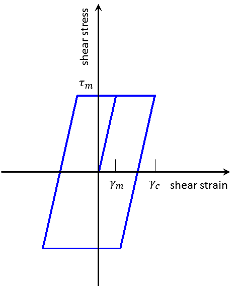
Figure 23: Shear stress/strain cycle—Mohr-Coulomb model.
The maximum stored energy, \(W\), during the cycle (assuming \(G\) represents an elastic modulus) is
and the dissipated energy (corresponding to the area enclosed by the loop) is
Hence,
Denoting the damping ratio by \(D\), and noting that for small values of \(D\) (Kolsky 1963),
or, substituting Equations (58) and (59) into Equation (61),
We plot normalized modulus (\(G/G_{max}\)) from Equation (57), and damping, \(D\), from Equation (59) against normalized cyclic strain, \(\gamma/\gamma_m\), in Equation (62). It can be seen that even a simple model (where “simple” is taken in the context of dynamics) exhibits an evolution of modulus and damping that can be matched to experimental results over limited ranges of cyclic strain.
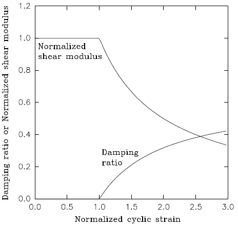
Figure 24: Modulus and damping ratio versus cyclic strain for elastic/plastic Mohr-Coulomb model.
Hysteretic Damping with the Linear Elastic Model
For the hysteretic damping model using the Hardin/Drnevich function described in Hysteretic Damping Formulation, Implementation, and Calibration, the backbone curve is given by
where \(\gamma_{ref}\) is the constant for the Hardin/Drnevich function. \(\gamma_{ref}\) is the ultimate value of \(\tau/G_{max}\):
This curve is followed for primary loading. For unloading/reloading, the Masing rule holds. For the case of cyclic shear loading at constant amplitude, \(\gamma_c\), the Masing rule gives, for unloading,
and for reloading,
where
The initial loading curve and loop traced in one cycle of unloading/reloading is sketched in Figure 25.
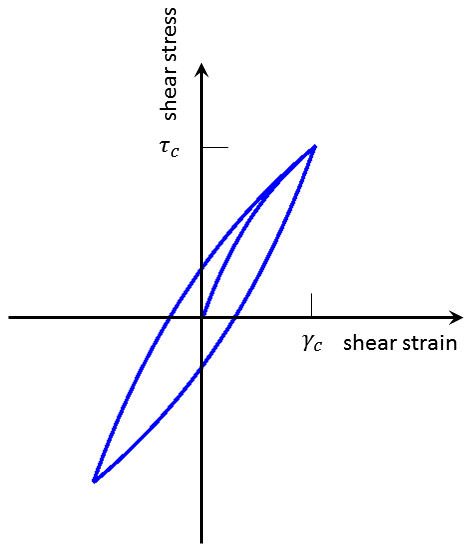
Figure 25: Shear stress/strain cycle—elastic model with Hardin/Drnevich hysteretic damping.
The energy dissipated in one full unloading-reloading cycle is given by the integral
After introduction of Equations (65) and (66) in Equation (68), and performing the integration, we obtain
The maximum stored energy in a cycle is
where \(\tau_c\) is given by Equation (67).
The damping ratio, \(D\), is obtained by combining Equations (68) and (69) with Equation (70):
Also, we note that application of l’Hospital rule gives
It is interesting to note that for the Hardin/Drnevich hysteretic damping and the elastic model, the damping ratio does not depend on \(G_{max}\). Also, \(D\) is larger for smaller values of \(\gamma_{ref}\). For an elastic, cyclic shear test of constant amplitude at constant volume, the use of hysteretic damping produces a response that is independent of the number of cycles performed.
Hysteretic Damping with the Mohr-Coulomb Model
When hysteretic damping is used with an elastic/plastic model in FLAC3D, the modulus-reduction technique is applied in the elastic range, and natural damping applies in the plastic range. In this case, we combine the Hardin/Drnevich hysteretic damping with a Mohr-Coulomb model. The Mohr-Coulomb model has a constant, tangent, elastic shear modulus, \(G_{max}\), and a constant yield stress, \(\tau_m\). The Hardin/Drnevich model is used to provide energy dissipation in the elastic range (but not to simulate yielding by means of a hyperbolic plasticity model). Accordingly, the yield level from the hyperbolic law must be higher than the Mohr-Coulomb yield stress. This will be the case provided that the following requirement is met:
where
An initial loading curve involving Mohr-Coulomb yielding and a loop traced in one cycle of unloading/reloading are sketched in Figure 26.
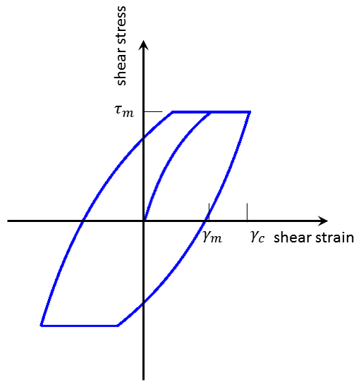
Figure 26: Shear stress/strain cycle—Mohr-Coulomb model with Hardin/Drnevich hysteretic damping.
The elastic range is defined by \(\gamma_c < \gamma_m\), where the shear strain, \(\gamma_m\), is found from the following relation (see Equation (63)):
In the elastic range, \(\gamma_c < \gamma_m\), the modulus reduction factor is given by Equation (63), or
In the plastic range, \(\gamma_c \ge \gamma_m\), the relation is
Also, in the plastic range, the energy dissipated in one cycle is the area enclosed by the loop in Equation (50). This energy may be expressed as the sum of two contributions:
where \(\Delta W_H\) is given by Equation (69)
and \(\Delta W_{MC}\) is expressed as (see Equation (59))
The maximum stored energy in one cycle is
and the damping ratio is
After substituting Equations (79) and (80) in Equation (82), we obtain with some manipulation,
The energy dissipation for the three damping cases is compared by exercising the equations for \(G/G_{max}\) and \(D\) over a cyclic strain range. A FISH function, listed in “datafiles\Dynamic\Damping-Compare\Damping-Compare.f3dat”, performs this exercise over a cyclic shear strain, \(\gamma_c\), from 0.0001 to 4.0. The value for \(\gamma_m\) is set to 0.01 and the value for \(\gamma_{ref}\) is set to 0.02. The results for \(G/G_{max}\) versus log \(\gamma_c/\gamma_m\), based upon Equations (57), (63), (76), and (77), are plotted in Figures 27. The results for \(D\) versus log \(\gamma_c/\gamma_m\), based upon Equations (62), (71), and (83), are plotted in Figure 28.
The inclusion of hysteretic damping is shown to reduce the shear modulus from the initial value of \(G_{max}\), and increase the damping ratio (compared to the elastic-only response). The damping ratio increases monotonically with shear strain amplitude and approaches the asymptotic value of \(2 / \pi\) for all three cases. The project file for this example can be found in “datafiles\Dynamic\Damping-Compare\Damping-Compare.f3prj”.
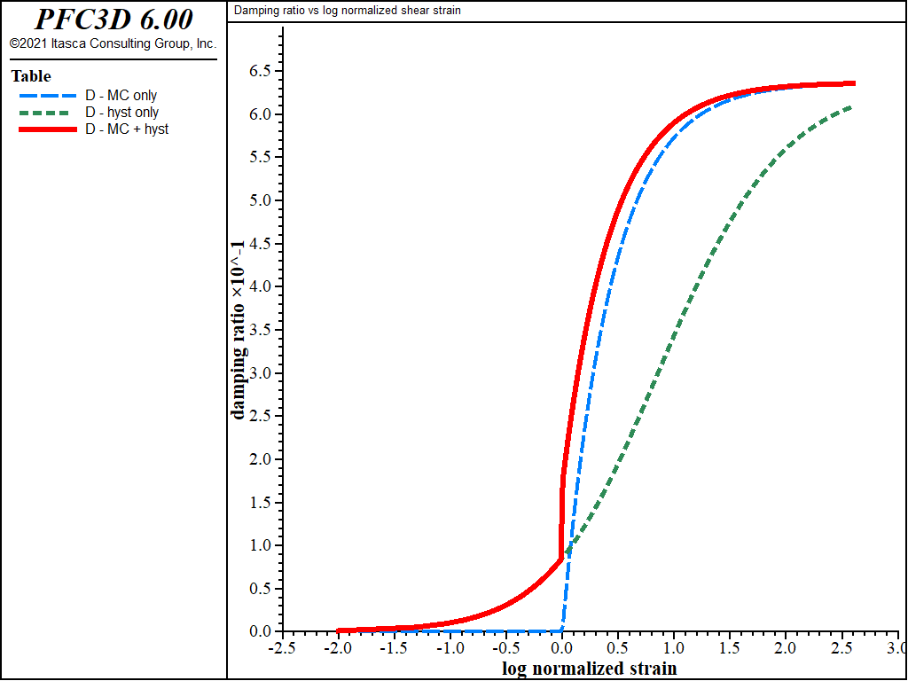
Figure 27: Normalized shear modulus vs log normalized shear stain for three damping cases.
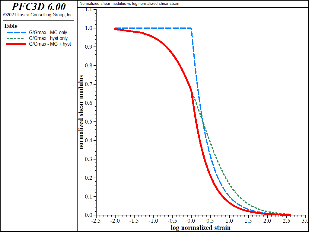
Figure 28: Damping ratio vs log normalized shear stain for three damping cases.
Dynamic Pore-Pressure Generation
Liquefaction Modeling
Liquefaction is defined as the loss of shear strength of soil under monotonic or cyclic loading, arising from a tendency for loose soil to compact under shear loading. The term “liquefaction” was originally coined by Mogami and Kubo (1953). Note that this definition covers both static and dynamic liquefaction; the effective stress does not necessarily have to be zero for a soil to liquefy. In particular, when a saturated cohesionless soil is submitted to rapid static or cyclic loading, the tendency for the soil to densify causes the effective stress to decrease, and the process leads to soil liquefaction.
It is known that pore pressures may build up considerably in some sands during cyclic shear loading. Eventually, this process may lead to liquefaction when the effective stress decreases. Although excess pore pressure is generally associated with liquefaction, it is not the direct cause of liquefaction. In constant volume tests with no applied load, it is the decrease in contact forces between particles that is responsible for the decrease in effective stress. The process is documented by Dinesh et al. (2004), who modeled similar tests (in which no change in pore pressure occurs) using the distinct element method. Alternatively, in undrained, simple shear tests under normal pressure, it is the irrecoverable reduction of porosity during cyclic compaction that generates pore pressure and, consequently, a decrease in effective stress.
Dilation plays an important role in the liquefaction process. As soil densifies under repeated shear cycles, grain rearrangement may be inhibited. Soil grains may then be forced to move up against adjacent soil particles, causing dilation to occur, the effective stress to increase and the pore pressure to decrease. Thus, densification is a self-limiting process.
The standard built-in constitutive models in FLAC3D do not model the liquefaction process directly. Coupled dynamic-groundwater flow calculations can be performed with FLAC3D. However, by default, the pore fluid simply responds to changes in pore volume caused by the mechanical dynamic loading; the average pore pressure remains essentially constant in the analysis.
There are many different models that attempt to account for pore pressure build-up, but they often do it in an ill-defined manner because they refer to specific laboratory tests. In a computer simulation, there will be arbitrary stress and strain paths. Consequently, an adequate model must be robust and general, with a formulation that is not couched in terms that apply only to specific tests. The following section describes a model that is simple, but that accounts for the basic physical process. In Comprehensive Liquefaction Constitutive Models, a review of more comprehensive models that have been developed is presented.
CS: Should this included file should be a link instead?
Simple Model Formulations
As mentioned in the previous section, in reality, pore pressure build-up is a secondary effect, although many people seem to think it is the primary response to cyclic loading. The primary effect is the irrecoverable volume contraction of the matrix of grains when a material is taken through a complete strain cycle with the confining stress held constant. Since it is grain rearrangement rather than grain volume change that takes place, the volume of the void space decreases under constant confining stress. If the voids are filled with fluid, then the pressure of the fluid increases and the effective stress acting on the grain matrix decreases. Note that pore pressures would not increase if the test were done at constant volume; it is the transfer of externally applied pressure from grains to fluid that accounts for the fluid-pressure increase.
Martin et al. Equation
This mechanism is well-described by Martin et al. (1975), who also note that the relation between irrecoverable volume-strain and cyclic shear-strain amplitude is independent of confining stress. They supply the following empirical equation that relates the increment of volume decrease per cycle of shear strain, \(\Delta\epsilon_{vd}\), to the cyclic shear-strain amplitude, \(\gamma\), where \(\gamma\) is presumed to be the “engineering” shear strain:
where \(C^c_1\), \(C^c_2\), \(C^c_3\), and \(C^c_4\) are constants.
Note
Note that these constants (\(C^c_1\), \(C^c_2\), \(C^c_3\), and \(C^c_4\)) are not identical to model input constants because the input applies to half cycle of shear strain.
Note that the equation involves the accumulated irrecoverable volume strain, \(\epsilon_{vd}\), in such a way that the increment in volume strain decreases as volume strain is accumulated. Presumably, \(\Delta\epsilon_{vd}\) should be zero if \(\gamma\) is zero; this implies that the constants are related as follows: \(C^c_1\ C^c_2\ C^c_4 = C^c_3\). Martin et al. (1975) then go on to compute the change in pore pressure by assuming certain moduli and boundary conditions (which are not clearly defined). We do not need to do this. Provided we correctly account for the irreversible volume change in the constitutive law, FLAC3D will take care of the other effects.
Byrne Equation
An alternative, and simpler, formula is proposed by Byrne (1991):
where \(C^c_1\) and \(C^c_2\) are constants with different interpretations from those of Equation (84). For Equation (85), Byrne (1991) notes that the constant, \(C^c_1\), can be derived from relative densities, \(D_r\), as follows:
Note
Note that these constants (\(C^c_1\) and \(C^c_2\)) are not identical to model input constants because the input applies to half cycle of shear strain.
Further, using an empirical relation between \(D_r\) and normalized standard penetration test values, \({(N_1)_{60}}\),
then
\(C^c_2\) is then calculated from \(C^c_2 = {0.4 / C^c_1}\), in this case. Refer to Byrne (1991) for more details.
The shear-induced volumetric strain for constant amplitude of cyclic shear strain predicted by this formula is plotted versus number of cycles in Figure 29. The formula predicts an increase in shear-induced (compactive) volumetric strain with the level of cyclic shear-strain. Also, for a given strain amplitude, \(\gamma\), the rate of accumulation decreases with the number of cycles.
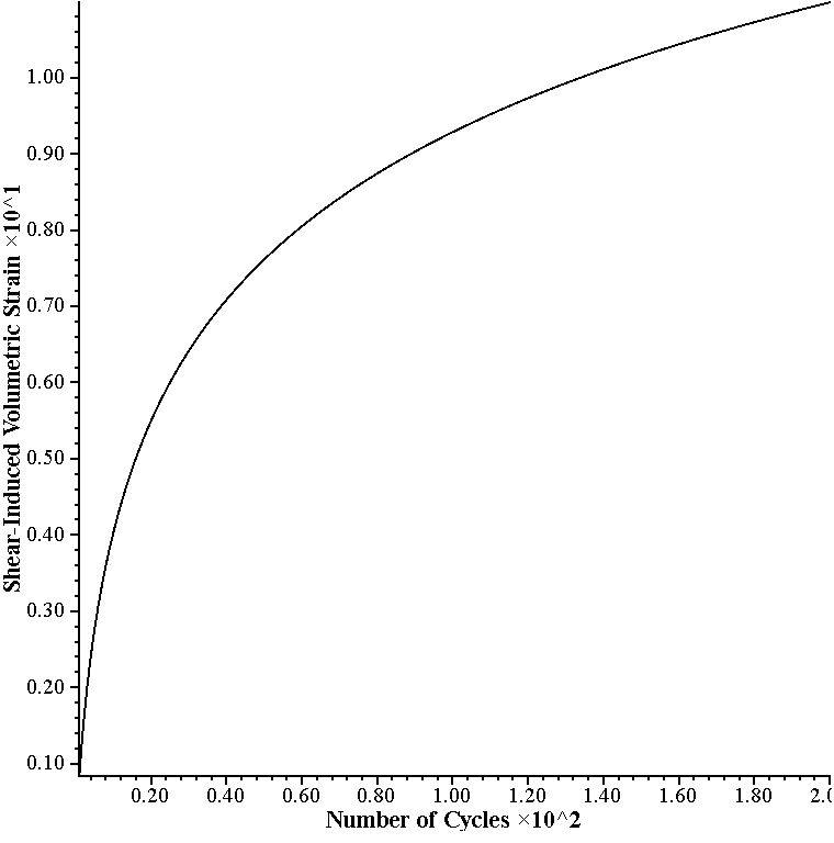
Figure 29: Finn/Byrne formula—constant, cyclic shear-strain amplitude.
The incremental volumetric behavior of the Finn/Byrne model (at the end of a cycle) may be expressed as
where \(\sigma_m = \sigma_{ii} / 3\) is the mean stress, \(p\) is pore pressure, \(\alpha\) is Biot coefficient (= 1 for soil), \(K\) is the drained bulk modulus of the soil and \(\epsilon\) is the volumetric strain. Note that \(\epsilon\) is positive in extension, while \(\epsilon_{vd}\) is positive in compression. For undrained conditions, the change in pore pressure is proportional to the change in volumetric strain:
where \(M\) is Biot modulus. After substitution of Equation (90) into (89), and solving for \(\Delta \epsilon\), we obtain
If the fluid is very stiff compared to the solid matrix (\(M>>>K\)), Equation (91) predicts no change in volume. Further, using \(\Delta \epsilon = 0\) in Equation (92) gives
Equation (92) predicts a decrease in magnitude of effective stress with cyclic shear strain (produced by an increase of shear induced compaction). Under conditions of constant stress, \(\Delta \sigma_m = 0\), there will be an increase in pore pressure that is proportional to the drained bulk modulus of the soil:
While under free stress conditions, the pore pressure will remain unchanged (\(\Delta p = 0\)), and the magnitude of the total stress will decrease according to
Note that in both situations, the drained (tangent) bulk modulus, \(K\), plays an important role in determining the magnitude of the cyclic loading impact on effective stress. The Finn/Byrne model, therefore, captures the main physics of liquefaction.
Finn Model
For a random pattern of strain cycles, it is appropriate to compute volumetric strains per half cycle (\({(\Delta \epsilon_{vd})}_{\rm 1/2 cycle}\)) — see, e.g., Byrne 1991. The Finn built-in constitutive model incorporates the following form of the Martin et al. and Byrne relations into the standard Mohr-Coulomb plasticity model:
Finn Model — Martin et al. Formulation
where \(C_1\), \(C_2\), \(C_3\) and \(C_4\) are model input constants.
Finn Model — Byrne Formulation
In addition to \(C_1\) and \(C_2\), a third model input parameter, \(C_3\), sets the threshold shear strain (i.e., the limiting shear-strain amplitude below which volumetric strain is not produced). The use of Equation (95) or (96) can be selected by setting parameter flag�_switch = 0 or 1, respectively. As it stands, the model captures the basic mechanisms that can lead to liquefaction in sand. In addition to the usual parameters (friction, moduli, etc.), the model needs the four constants for Equation (95), or three constants for Equation (95). For Equation (84), Martin et al. (1975) describe how these may be determined from a drained cyclic test. Alternatively, one may imagine using some trial values to model an undrained test with FLAC3D, and compare the results with a corresponding laboratory test; the constants could then be adjusted to obtain a better match.
Note that following Byrne (1991), the input parameters \(C_1\) and \(C_2\) are related to relative density or blow count as follows:
where \(C^c_1\) is given by Equation (86) or Equation (88), respectively.
In the Finn model, there is logic to detect a strain reversal in the general case. In Martin et al. (1975) (and most other papers on this topic), the notion of a strain reversal is clear, because they consider one-dimensional measures of strain. In a three-dimensional analysis, however, there are at least six components of the strain-rate tensor. The six strain measures are accumulated in the Finn model in FLAC3D as follows:
We use the following scheme to locate extreme points in strain space. Denoting the previous point by superscript (°), and the one before that with (°°), the previous unit vector, \(n_i^\circ\), in strain space is computed:
where subscript \(i\) takes the values 1 to 6, and repeated indices imply summation.
The projection \(d\) of the new vector, \(\epsilon_i - \epsilon_i^{\circ}\), from the old point to the new point is given by the dot product of the new vector with the previous unit vector,
We use the rule that \(d\) must be negative (so that the new strain segment corresponds to a reversal compared to the previous segment). We then monitor the absolute value of \(d\) and make the following calculation when it passes through a maximum, \(d_{\rm max}\), provided that a minimum number of timesteps has elapsed (to prevent the reversal logic being triggered again on transients that immediately follow a reversal). This threshold number of timesteps is controlled by the property named ff�_latency, which is set to 50.0 in the runs reported here.
Having obtained the engineering shear strain, \(\gamma\), we insert it into Equation (95) or (96) and obtain \({(\Delta \epsilon_{vd})}_{\rm 1/2 cycle}\). We then update \(\epsilon_{vd}\), as follows, and save it for use in Equation (95) or (96).
We also save one-third of \({(\Delta \epsilon_{vd})}_{\rm 1/2 cycle}\) and revise the direct strain increments input to the model at the next half cycle:
Note that FLAC3D’s compressive strain increments are negative and \(\Delta \epsilon_{vd}\) is positive. Hence, the mean effective stress decreases.
The logic described above is certainly not perfect, but it seems to work in simple cases. However, the user must verify that the algorithm is appropriate before applying it to real cases. In particular, the number of “half cycles” detected strongly depends on the relative magnitude of horizontal and vertical motion. Hence, the rate of build-up of pore pressure will also be sensitive to this ratio. It may be more practical to consider just the shear components of strain for something like a dam, which is wide compared to its height. Ultimately, we need better experimental data for volume changes during complicated loading paths; the model should then be revised accordingly. One effect that has been shown to be very important (see, for example, Arthur et al. 1980) is the effect of rotation of principal axes: volume compaction may occur even though the magnitude of deviatoric strain (or stress) is kept constant. Such rotations of axes occur frequently in earthquake situations. Another effect that is not incorporated into the Finn model is that of modulus increase induced by compaction—it is known that sand becomes stiffer elastically when compaction occurs by cyclic loading. This modification could be incorporated by using the UDM option.
The Finn model is loaded in FLAC3D with the zone cmodel command
(i.e., zone cmodel assign finn).
The code must be configured for dynamic analysis (model configure dynamic) to apply the model.
As with the other built-in models, the properties are assigned with the zone property command.
The following keywords are used to assign properties for the Finn model:
finn Model Properties
Use the following keywords with the zone property command to set these properties of the Finn model.
- finn
- bulk f
elastic bulk modulus, \(K\)
- cohesion f
cohesion, \(c\)
- constant-1 f
constant, \(C_1\)
- constant-2 f
constant, \(C_2\)
- constant-3 f
constant, \(C_3\)
- constant-4 f
constant, \(C_4\)
- friction f
internal angle of friction, \(\phi\)
- poisson f
Poisson’s ratio, \(\nu\)
- shear f
elastic shear modulus, \(G\)
- young f
Young’s modulus, \(E\)
- flag-brittle b
[advanced] if true, the tension limit is set to 0 in the event of tensile failure. The default is false.
- table-cohesion s
[advanced] name of the table relating cohesion to plastic shear strain
- table_dilation s
[advanced] name of the table relating dilation angle to plastic shear strain
- table-friction s
[advanced] name of the table relating friction angle to plastic shear strain
- table-tension s
[advanced] name of the table relating tension limit to plastic tensile strain
- number-count i
[read only] number of shear strain reversals (half cycles) detected
- strain-shear-plastic f
[read only] accumulated plastic shear strain
- strain-tensile-plastic f
[read only] accumulated plastic tensile strain
- strain-volumetric-irrecoverable f
[read only] accumulated irrecoverable volume strain, \(\epsilon_{vd}\), which is positive in compression, an interval variable used in Martin et al and Byrne formula
- Notes:
- Only one of the two options is required to define the elasticity: bulk modulus \(K\) and shear modulus \(G\), or Young’s modulus \(E\) and Poisson’s ratio \(\nu\). When choosing the latter, Young’s modulus \(E\) must be assigned in advance of Poisson’s ratio \(\nu\).
- The tension cut-off is \({\sigma}^t = min({\sigma}^t, k_{\phi} / q_{\psi})\).
Footnotes
Advanced properties have default values and do not require specification for simpler applications of the model.
Read only properties cannot be set by the user. However, they may be listed, plotted, or accessed through FISH.
Simulation of the Liquefaction of a Layer
The material constants in the Finn that control pore pressure build-up are related to the volumetric response in a drained test. However, if results are available for an undrained test, then the test itself may be modeled with FLAC3D, and the material constants deduced by comparing the FLAC3D results with the experimental observations. Some adjustment will be necessary before a match is found.
In the following example, a “shaking table” is modeled with FLAC3D.
Comprehensive Liquefaction Constitutive Models
The state of practice for seismic analysis involving liquefiable materials is currently experiencing a shift from using empirical schemes (first developed in the 1970s) to simulate liquefaction, to time-marching numerical methods incorporating liquefaction constitutive models currently at various stages of development. There are several ways liquefaction behavior is included in numerical methods, ranging from total-stress empirical schemes to estimate liquefaction conditions (e.g., the UBCTOT model—see Beaty and Byrne 2000), to simple effective-stress shear-volume coupling schemes (e.g., the Finn model, and the “Roth” model—see Dawson et al. 2001), to more comprehensive constitutive models (e.g., the UBCSAND model—see Byrne et al. 1995; and bounding surface models such as the model described in Wang 1990, and the model described in Papadimitriou et al. 2001) that address cyclic shearing via kinematic hardening.
To help practicing engineers choose a procedure best suited to their needs, a selection of approaches is outlined below, ranging from simple to elaborate in terms of complexity and model parameter determination. This is not a comprehensive list, but is a selection that illustrates the different types of liquefaction models that have been developed and used in two-dimensional FLAC, and could be used in FLAC3D. [3] One important factor to keep in mind is that, in engineering practice, the use of a very complicated model for liquefaction analyses is often hardly justified, considering the many uncertainties with respect to soil properties and earthquake motions, and the numerous approximations that must be made (see Dawson et al. 2001). Before describing the individual models, it will be helpful to review the current state of practice for liquefaction analysis. (See Byrne et al. 2006 for further discussion on state-of-practice analysis.)
State of Practice — The standard practice approach for liquefaction analysis of earthquake loading is based on a total-stress analysis in which it is assumed that the liquefiable soil remains undrained at the in-situ void ratio (Byrne and Wijewickreme 2006). Typically, this analysis approach is divided into three steps:
- Triggering Evaluation: Typically, an equivalent-linear elastic, dynamic analysis (such as SHAKE) using strain-compatible moduli and damping is conducted for the design earthquake. The cyclic stress ratio (CSR) [4] is evaluated from the numerical simulation and compared to the value of the cyclic stress resistance that the soil has because of its density (CRR) [5], derived from empirical curves. A factor of safety against triggering liquefaction is evaluated using the ratio of CRR and CSR (e.g., see Byrne and Anderson 1991, and Youd et al. 2001).
- Flow Slide Assessment: Post-liquefaction (undrained) strengths are assigned in zones predicted to liquefy from the triggering evaluation analysis, and a standard limit-equilibrium analysis is carried out to evaluate the factor of safety against a flow slide. Post liquefaction strengths may be derived from penetration resistance (corrected blow count \((N_1)_{60}\)) using empirical charts (e.g., see Seed and Harder 1990, and Olson and Stark 2002).
- Seismic Displacements: Displacements are evaluated using the Newmark approach (see Newmark 1965). In this step, the potential sliding block of soil is modeled as a rigid mass resting on an inclined plane. The design time history of acceleration is applied at the base, and the equation of motion is solved to obtain the displacement of the mass caused by the shaking.
The main shortcomings of the standard practice approach are that the three aspects of liquefaction (triggering, flow slide, and deformation) are treated sequentially, when in reality they may interact locally in various zones of the soil structure and affect the overall behavior of the soil mass. Also, no direct account is made of excess pore-pressure redistribution and dissipation.
Total-Stress Synthesized Procedure
The synthesized procedure of Beaty and Byrne (2000) uses FLAC and the UBCTOT constitutive model to combine the three steps of the standard practice approach (triggering, flow slide, and estimate of liquefaction-induced displacements) into one single analysis. The procedure, which assumes undrained behavior, uses a (two-dimensional) total-stress approach to liquefaction analysis and relies on adjustment of liquefied element properties (stiffness and strength) at the instant of triggering of liquefaction. The main features of the UBCTOT model are summarized below.
A seismic analysis using the synthesized procedure starts from a static state of equilibrium for the FLAC model. The seismic analysis is conducted in total-stress space. UBCTOT uses Mohr-Coulomb elasto-plastic logic with zero friction and a value of cohesion equal to the undrained shear strength, in combination with Rayleigh damping. The elastic shear modulus is assigned a value of \(G_{max}\) multiplied by a modulus reduction factor (MRF). Unlike equivalent-linear methods, this approach is not iterative, and appropriate values of MRF and damping are selected at the start of the seismic analysis. Triggering of liquefaction is based on changes of shear stress on the horizontal plane, \(\tau_{xy}\). The irregular shear-stress history caused by the earthquake is interpreted in each FLAC zone as a succession of half-cycles with the contribution to triggering determined by the maximum value of \(\tau_{cyc}\), defined as the difference between \(\tau_{xy}\) and the initial horizontal shear-stress prior to earthquake loading (i.e., the static bias). A cumulative damage approach is used to combine the effects of each half-cycle. The approach converts the nonuniform history into an equivalent series of uniform stress cycles with amplitude equal to \(\tau_{15}\) (i.e., the value of \(\tau_{cyc}\) required to cause liquefaction in 15 cycles, which is approximately the number of cycles in a magnitude 7.5 earthquake). This is done using an empirical chart giving the cyclic stress ratio (CSR) versus cycles to liquefaction. Several property changes are imposed when liquefaction is detected in a FLAC zone: a residual shear strength is assigned; a reduced loading stiffness is used; and unloading uses a stiffer modulus than loading, according to a bilinear stiffness model. Also, a hydrostatic stress state is imposed when a zone experiences a shear-stress reversal. Finally, reduced viscous damping is assigned in a liquefied zone. The constitutive model also has logic to account for anisotropy in stiffness and strength. See Beaty (2001) for additional information.
The UBCTOT model removes some of the limitations associated with the sequential approach to problem solving used in the state-of-practice procedure, while relying on similar empirical charts for triggering of liquefaction and residual strength.
- The following are some of the drawbacks of the model:
- the use of equivalent modulus ratio that may not capture the pre-liquefaction phase well;
- the cyclic shear stresses are accounted for on the horizontal plane only;
- the simplified manner in which the undrained shear strength is specified;
- pore pressure is not taken into account explicitly; and
- liquefaction due to monotonic loading is not considered.
Loosely Coupled Effective-Stress Procedure
The Roth model is a loosely coupled effective-stress constitutive model to generate pore pressure from shear stress cycles using the Seed cyclic stress approach (Seed and Idriss 1971). This model is built around the standard FLAC Mohr-Coulomb model. The (two-dimensional) model counts shear stress cycles by tracking the shear stress acting on horizontal planes (\(\tau_{xy}\)) and looking for stress reversals. The cyclic stress ratio (CSR) of each cycle is measured, and this is used to compute the incremental “damage” that is then translated into an increment of excess pore pressure. The procedure is “loosely coupled” because pore pressures are only computed after each 1/2 cycle of strain or stress as the analysis proceeds. The model incorporates residual strength (a critical parameter for seismic stability analyses) by using a two-segment failure envelope consisting of a residual cohesion value and zero friction angle that is extended to meet with the traditional Mohr-Coulomb failure envelope.
The model is simple, robust, and practice-oriented; it is based on the widely accepted cyclic-stress approach with input parameters readily obtainable from routine field investigations. (Note that liquefaction due to monotonic loading is not considered.) A disadvantage of the model is that liquefaction-induced consolidation settlements are not captured, because the actual physical mechanism of liquefaction, whereby pore pressure is generated through contraction of the soil skeleton, is bypassed. The model is applicable to problems where slope movements due to reduced shear strength are the main concern (such as seismic stability of dams and waterfront retaining structures), while shaking-induced consolidation settlements are of secondary importance. See Roth et al. (1991), Inel et al. (1993), Roth et al. (1993), and Perlea et al. (2008) for some field applications.
The Roth model is similar to the built-in Finn model, which is also considered a loosely coupled effective-stress model. The primary difference is that in the Finn model, the volumetric strains induced by cyclic loading are evaluated based on an experimental curve of irrecoverable volumetric strain versus number of constant amplitude cycles. Pore pressures are then generated from these volumetric strains, as well as from contraction of the soil skeleton. Also, the Finn model in FLAC (and FLAC3D ), at present, does not include a post-liquefaction residual strength.
Fully Coupled Effective-Stress Procedure
The UBCSAND model is a fully coupled (kinematic hardening) effective-stress constitutive model to predict seismic response and liquefaction of cohesionless soils in plane strain problems. The model uses an elasto-plastic formulation based on an assumed hyperbolic relation between stress ratio and plastic shear strain, similar to the Duncan and Chang (1970) formulation. It is applicable for monotonic as well as cyclic loading (e.g., see Byrne et al. 2003, 2006).
The model implementation is a modified form of the built-in Mohr-Coulomb model in FLAC that accounts for a strain-hardening frictional behavior, neglects cohesion, and applies to plane strain conditions. The hardening law is a hyperbolic function of plastic shear strain. Unloading is assumed to be nonlinear elastic, with bulk and shear modulus as functions of mean (in-plane) effective stress. Stress reversal is detected by a change of sign in horizontal shear stress, \(\tau_{xy}\). Reloading is elasto-plastic, with the yield locus reset to the value at the reversal point. Plastic flow is nonassociated; the logic is based on a variation of Rowe’s stress-dilatancy theory. According to this theory, there is a constant-volume stress ratio, \(\phi_{cv}\), below which the material contracts (i.e., for mobilized friction, \(\phi_m\), smaller than \(\phi_{cv}\)), while for higher stress ratios (i.e., for \(\phi_m > \phi_{cv}\)), the material dilates. The effect of relative density is addressed through the choice of material properties. Most properties are calibrated to field experience as well as centrifuge tests and are conveniently related to blow count, \((N_1)_{60}\).
The model is able to capture the stiff pre-liquefaction stage, the onset of liquefaction at the appropriate number of cycles, and the much softer post-liquefaction response observed in cyclic, simple shear-constant volume tests.
The coupled effective-stress approach corrects many drawbacks of the previous approaches. Although most parameters are related to blow count and rely on a growing body of data and experience, it is always good practice to check on model parameters for each layer (using numerical simulation of a simple shear test) to verify that if it has to liquefy in \(N\) cycles according to the field data during dynamic loading, it will. Also, because comparison with standard procedures may not be straightforward, it is recommended that the model be used under the supervision of an experienced practitioner. With time, and with the increase of its usage, the model should become more prominent and be used for problems ranging from simple to complex with little effort.
The primary disadvantages are: 1) the logic for detection of stress reversal is based on horizontal shear stress only; and 2) the present formulation applies only to two-dimensional analysis.
Fully Coupled Effective-Stress Bounding-Surface Procedure
Bounding surface plasticity provides a framework to account for cyclic stress reversal in two and three dimensions (see Dafalias 1986, and Wang 1990). The models developed by Wang (1990) (herein named the WANG model) and Papadimitriou et al. (2001) (herein named the PAPADIMITRIOU model) are two (kinematic-hardening) constitutive models that have been implemented in FLAC based on that logic.
WANG Model — The WANG model is an effective stress, bounding-surface hypoplasticity model for (cohesionless) soil that is capable of reproducing, in detail, typical monotonic and cyclic, drained and undrained, hardening and softening behavior observed in classical laboratory tests on initially dense and loose soils (Wang 1990). (The term hypoplasticity characterizes the dependence of loading and plastic strain-rate directions on stress-rate direction.)
The model formulation includes a noncircular pyramidal failure (bounding) surface, a loading surface, a surface of phase transformation (at which contractive behavior changes to dilative during shearing), and a critical state surface (defining an ultimate state in which the sand deforms at constant volume under constant stress). The three-dimensional effective-stress model requires the specification of 15 constants for a given sand (eight parameters are required for two-dimensional analysis). One disadvantage is that model calibration is an arduous task because most model constants are not related to properties with which the practitioner is familiar, and the body of available parameter data is not yet sufficiently well-developed. Also, comparison to state-of-practice analysis is not straightforward. The relation between cyclic stress ratio, number of cycles to liquefaction and normalized blow count can be used to calibrate the model (Wang et al. 2001), but there is no direct relation between empirical rules used in standard practice and theoretical laws used in the model theory. The WANG model is a sophisticated research tool for laboratory-scale experiments. Application of the model to study boundary-value problems at the field scale should probably not be attempted without the advice of the model developer, whose assistance may be required for model calibration, interpretation of results, and support on possible issues with numerical implementation.
PAPADIMITRIOU Model — The PAPADIMITRIOU model is an effective stress, bounding-surface model for loose and dense sand that is based on critical state elasto-plasticity (Papadimitriou et al. 2001, Papadimitriou and Bouckovalas 2002). The model applies to monotonic as well as cyclic loading (in two and three dimensions) of non-cohesive soils under small and large strains. The model uses a kinematic hardening noncircular cone as the (loading) yield surface. In addition to bounding and dilatancy (marking the transition between contractive and dilatants behavior) surfaces, the model also contains a critical-state surface (defining an ultimate state in which the sand deforms at constant volume under a constant shear and confining stress). The model contains a total of 14 parameters: 11 of the parameters can be derived from in-situ and laboratory tests, while the remaining three must be derived indirectly via trial-and-error simulations of drained and undrained laboratory tests. (Note that each parameter set is independent of initial and drainage conditions, as well as cyclic shear-strain amplitude.)
The model has the capability to reproduce, qualitatively, the characteristic behavior observed in cyclic experiments, including the degradation of shear modulus and increase of hysteretic damping with cyclic shear strain amplitude, the shear and volumetric strain accumulation at a decreasing rate with increasing number of cycles, and the increase in liquefaction resistance with density. Comparisons with centrifuge experiments have been made (Andrianopoulos et al. 2006a), and the ability of the model to study a practical problem of geotechnical earthquake engineering has been demonstrated (Andrianopoulos et al. 2006b). The disadvantages are the model calibration, which is a rather tedious procedure and requires a test database not readily available in most cases, and the long computational time required for the solution of practical problems. Also, comparison to standard practice is not straightforward. Application of the model to study boundary-value problems at the field scale is not recommended at this time without the assistance of the model developer for model calibration, interpretation of results, and eventual support for issues related to numerical implementation.
| [1] | This section is abstracted with permission from the publication by Mejia and Dawson (2006). |
| [2] | A spectral analysis based on a fast Fourier transform is supplied as a FISH function in the FISH library in “datafiles\FISH\Library\fft.fis”. |
| [3] | The liquefaction models discussed in this section have been implemented in two-dimensional FLAC either as FISH or C++ user-defined constitutive models. (Contact the authors of these liquefaction models in order to receive additional information about the model or to inquire about receiving a copy of the model.) Itasca does not provide technical support for these models. |
| [4] | Cyclic Stress Ratio: Ratio of maximum dynamic shear stress to the initial vertical effective stress prior to the earthquake at a specific location. |
| [5] | Cyclic Resistance Ratio: Commonly taken as the value of CSR that causes liquefaction in 15 cycles of dynamic loading. |
⇐ Shear Wave On Stiff Wall In Soft Soil: Dynamic Multi-Stepping | Shear Wave Propagation in a Vertical Bar ⇒
| Was this helpful? ... | PFC 6.0 © 2019, Itasca | Updated: Nov 19, 2021 |