Grid Discretization

Among three-dimensional constant strain-rate elements, tetrahedra have the advantage of not generating hourglass deformations (i.e., deformation patterns created by combinations of nodal velocities producing no strain rate, and thus no nodal force increments). However, when used in the framework of plasticity, these elements do not provide for enough modes of deformation (see Nagtegaal et al. 1974). In particular situations, for example, they cannot deform individually without change of volume as required by certain important constitutive laws. In those cases, the elements are known to exhibit an overly stiff response compared to what is expected from theory. To overcome this problem, a process of mixed discretization is applied in FLAC3D.

The principle of the mixed discretization technique is to give the element more volumetric flexibility by proper adjustment of the first invariant of the tetrahedra strain-rate tensor. [*] Application of the technique differs depending on whether primary discretization of the body is done into hexahedral zones or into tetrahedra. In the approach pioneered by Marti and Cundall (1982), a coarser discretization in zones is superposed to the tetrahedral discretization, and the first strain-rate invariant of a particular tetrahedron in a zone is evaluated as the volumetric-average value over all tetrahedra in the zone. The method is illustrated in Figure 1. In the particular mode of deformation sketched there, individual constant strain-rate elements will experience a volume change incompatible with a theory of incompressible plastic flow. In this example, however, the volume of the assembly of tetrahedra (i.e., the zone) remains constant, and application of the mixed discretization process allows each individual tetrahedron to reflect this property of the zone, hence reconciling its behavior with that predicted by the theory.

Mixed Discretization for a Hexahedral Grid

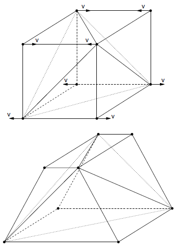
Figure 1: Mode of deformation for which mixed discretization would be most efficient.

In FLAC3D, a zone corresponds to an assembly of nt tetrahedra, as illustrated in Figure 2 for the case nt = 5. Consider a particular zone where the strain-rate tensor of a tetrahedron locally labeled l in that zone is first estimated, and then decomposed into deviatoric and volumetric parts:

(1)\[ {\xi}_{ij}^{[l]} = {\eta}_{ij}^{[l]} + {{{\xi}^{[l]}}\over{3}}{\delta}_{ij}\]

where η[l] is the deviatoric strain-rate tensor, and ξ[l] is the strain-rate first invariant,

(2)\[ {\xi}^{[l]} = {\xi}_{ii}^{[l]}\]

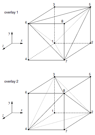
Figure 2: An 8-node zone with 2 overlays of 5 tetrahedra in each overlay.

The first invariant for the zone is then calculated as the volumetric average value of the first invariant over all tetrahedra in the zone:

(3)\[ {\xi}^z = {{\sum_{k=1}^{n_t} {\xi}^{[k]} V^{[k]}}\over{\sum_{k=1}^{n_t}V^{[k]}}}\]

where V[k] is the volume of tetrahedron k. F inally, the tetrahedron strain-rate tensor components are calculated from

(4)\[ {\xi}_{ij}^{[l]} = {\eta}_{ij}^{[l]} + {{{\xi}^z}\over{3}} {\delta}_{ij}\]

Dilatant constitutive laws will produce changes in mean normal stress when yielding occurs. For a consistent technique, the first invariant of the stress tensor, derived after application of the strain-rate increment, must also be evaluated as a volumetric average for the zone. In this process, the stress tensor of a particular tetrahedron l in a zone is first estimated and decomposed into deviatoric and volumetric parts:

(5)\[ {\sigma}_{ij}^{[l]} = s_{ij}^{[l]} + {\sigma}^{[l]} {\delta}_{ij}\]

where [s][l] is the deviatoric strain-rate tensor, and σ[l] is the mean normal stress.

(6)\[ {\sigma}^{[l]} = {{1}\over{3}} {\sigma}_{ii}^{[l]}\]

The first invariant for the zone is calculated as the volumetric average value over all tetrahedra in the zone:

(7)\[ {\sigma}^z = {{\sum_{k=1}^{n_t}{\sigma}^{[k]} V^{[k]}}\over{\sum_{k=1}^{n_t}V^{[k]}}}\]

Finally, the tetrahedron stress-rate tensor components are calculated using

(8)\[ {\sigma}_{ij}^{[l]} = s_{ij}^{[l]} + {\sigma}^z {\delta}_{ij}\]

In FLAC3D, the discretization process starts with the coarser grid: zones are defined and then discretized (internally) into tetrahedra. An eight-noded zone, for instance, can be discretized into two (and only two) different configurations of five tetrahedra (corresponding to overlay 1 and 2 in Figure 2. The calculation of nodal forces (based on evaluation of strain rates and stresses) can be carried out using one overlay or a combination of two overlays. The advantage of the two-overlay approach is to ensure symmetric zone response for symmetric loading. In this case, mixed discretization is carried out over the combination of two overlays, and nodal forces computations are evaluated by averaging over the two overlays.

Nodal Mixed Discretization for a Tetrahedral Grid

Nodal mixed discretization (NMD) is a variation on the mixed discretization scheme, in which averaging of the volumetric behavior is carried out on a node basis instead of a zone basis. The procedure is applied on the triangle or tetrahedral-based mesh; it does not require the assembly of elements into zones. Also, the constitutive model is called on an element basis, as usual (no call is made on a node basis for the volumetric behavior, as in the average nodal pressure (ANP) formulation described by Bonet and Burton 1998). The procedure involves a nodal mixed discretization on strain, and one on stress. Both steps are considered below.

First we recall the general calculation sequence embodied in FLAC and FLAC3D:

1. Nodal forces are calculated from stresses, applied loads and body forces (velocity and displacement vary linearly; stress and strain are constant within an element).
2. The equations of motion are invoked to derive new nodal velocities and displacements.
3. Element strain rates are derived from nodal velocities.
4. New stresses are derived from strain rates, using the material constitutive law.

In the NMD technique, the calculation sequence is respected. However, an averaging procedure is carried out on strain rates (end of step 3) and on stress increments (end of step 4), as described below.

Nodal mixed discretization on strain

The strain rate \(\dot \varepsilon_{ij}\) is derived from nodal velocities, as usual. The strain rate is then partitioned into deviatoric, \(\dot e_{ij}\), and volumetric, \(\dot e\), components:

(9)\[ \dot \varepsilon_{ij} = \dot e_{ij} + \dot e \delta_{ij}\]

where \(\delta_{ij}\) is the Kroenecker delta.

A nodal volumetric strain rate (defined as the weighted average of the surrounding element values) is calculated using the formula

(10)\[ \dot e_n = {{\sum_{e = 1}^{m_n} \dot e_e V_e} \over {\sum_{e = 1}^{m_n} V_e}}\]

where mn are the elements surrounding node n, and Ve is the volume of element e.

After nodal volumetric strain rate values are obtained, a mean value for the element \(\bar{\dot e}\) is calculated by taking the average of nodal values:

(11)\[ {\bar{\dot e}} = {1 \over d} \sum_{n = 1}^{d} \dot e_n\]

where d = 3 for a triangle and 4 for a tetrahedral.

Finally, the element strain rate is redefined by superposition of the deviatoric part and volumetric average:

(12)\[ \dot \varepsilon_{ij} = \dot e_{ij} + \bar{\dot e} \delta_{ij}\]

The constitutive model is called to derive new stresses (from strain rates) and previous stresses.

Nodal mixed discretization on stress

Consider an incremental volumetric constitutive stress-strain law which, for small increments, can be linearized in the form

(13)\[ \dot \sigma = K({\bar{\dot e}} - {\dot e^p})\]

where \(\dot e^p\) stands for plastic volumetric strain increment, and the value is nonzero for dilatant/hfilbreak contractant material. The associated nodal forces must be consistent with the assumptions made to define the element kinematics. To enforce this, a nodal mixed discretization procedure is applied on the term \(K\dot e^p\), as described below. For convenience, we refer to the term \(K\dot e^p\) as \(\dot \sigma^p\); With this convention, Equation (13) may be expressed as

(14)\[ \dot \sigma = K{\bar{\dot e}} - \dot \sigma^p\]

The value \(\dot \sigma^p\) is a standard quantity evaluated in the constitutive model procedure.

The technique for nodal mixed discretization on stress is similar to the one applied for strain. First, nodal values for \(\dot \sigma^p\) are calculated as the weighted average of the surrounding element values:

(15)\[ \dot \sigma_n^p = {{\sum_{e = 1}^{m_n} \dot \sigma^p V_e} \over {\sum_{e = 1}^{m_n} V_e}}\]

After the nodal values \(\dot \sigma_n^p\) are obtained, a mean value for the element \(\bar{\dot{\sigma}}^p\) is calculated by taking the average of nodal values:

(16)\[ \bar{\dot{\sigma}}^p = {1 \over d} \sum_{n = 1}^d \dot \sigma_n^p\]

where, again, d = 3 for a triangle and 4 for a tetrahedra.

Finally, the stresses calculated by the constitutive model are corrected by substituting \(\bar{\dot{\sigma}}^p\) for \(\dot \sigma^p\) in the returned value:

(17)\[ \sigma_{ij} => \sigma_{ij} + (\dot \sigma^p - \bar{\dot{\sigma}}^p) \delta_{ij}\]

Clearly, the nodal mixed discretization on stress will only be relevant for dilatant/contractant materials.

It is important to note that the averaging manipulations involved in the NMD technique are done independent of the constitutive model formulation, which remains unaffected. (The plastic volumetric “stress correction” \(\dot \sigma^p\) calculated by the constitutive model is simply passed back from the constitutive model as one of the state variables.)

Also, because of the way the averaging procedure is carried out, the resulting tetrahedral formulation gives the correct behavior in patch test situations where \(\dot \sigma\) is uniform, and thus equal, for all elements.

The nodal averaging procedure involved in the NMD technique removes the excessively constrained kinematics of the linear velocity element.

[*]	This invariant gives a measure of the rate of dilation of the constant strain-rate tetrahedron.