FLAC3D Theory and Background • Fluid-Mechanical Interaction

Consolidation Settlement at the Center of a Strip Load

Note

To view this project in FLAC3D, use the menu command Help ‣ Examples…. Choose “Fluid/ ConsolidationSettlement” and select “ConsolidationSettlement.f3dprj” to load. The project’s main data files are shown at the end of this example.

The prediction of the time settlement of foundations on soft saturated soil is a problem of wide practical interest in soil mechanics. The fluid can in general be considered as incompressible compared to the soil matrix for the simulations, and thus this type of problem is ideal for testing the saturated fast-flow scheme in FLAC3D, described in Fully Saturated Fast Flow. This verification problem involves the consolidation settlement produced by a uniform strip loading on a semi-infinite elastic medium, which is free to drain at the surface.

The two-dimensional poro-elastic problem of a semi-infinite stratum loaded on the plane \(z\) = 10 by a uniform normal pressure, \(P\), along the strip \(-a \le x \le a\) has been analyzed by McNamee and Gibson (1960). The fluid is assumed to be incompressible in their solution. The case in which the pore pressure vanishes at \(z\) = 10 (i.e., a completely permeable surface) is considered. The consolidation surface settlement for the special case of zero Poisson’s ratio is given by the closed form solution

(1)\[{\hat{u}-\hat{u}_{und}} = {{\chi{_1} + \chi{_2}} \over 2\hat{G}}\]

where

(2)\[\chi{_1} = \sqrt{\tau \over \pi} \biggl[erf ({{1+\hat{x}} \over {2\sqrt{\tau}}}) + erf ({{1-\hat{x}} \over {2\sqrt{\tau}}}) \biggr]\]

(3)\[\chi{_2} = {1 \over 2\pi} \biggl[(1 + \hat{x}) E_1 \bigl[{({1+\hat{x}})^2 \over {4\tau}}\bigr] + (1 - \hat{x}) E_1 \bigl[{({1-\hat{x}})^2 \over {4\tau}}\bigr] \biggr]\]

\(\hat{u}\) and \(\hat{u}_{und}\) are the nondimensional total vertical displacement and undrained vertical displacement, respectively, at \(z\) = 0. \(\hat{x}\) is the nondimensional horizontal distance, and \(\hat{G}\) is the nondimensional shear modulus. These quantities are defined:

(4)\[\hat{u} = {u_z \over a}, \hat{x} = {x \over a}, \hat{G} = {G \over P}\]

where \(u_z\) is the vertical displacement, and \(G\) is the shear modulus.

erf is the error function and \(E_1\) is the exponential integral. \(\tau\) is a dimensionless time parameter, given as

(5)\[{{\tau} = {{c_v t} \over a^2}}\]

where \(c_v\) is the scaled diffusivity, and \(t\) is time. For zero Poisson’s ratio, \(c_v\) is defined as

(6)\[{c_v = 2 G k}\]

where \(k\) is the mobility coefficient.

For the numerical simulation with FLAC3D, \(a\) = 1, \(\hat{G}\) = 0.5, \(P\) = 1, and \(c_v\) = 1. The problem conditions are simulated under plane-strain conditions, and advantage is taken of the problem geometry half-symmetry.

The FLAC3D model grid used for this analysis is shown in Figure 1. The grid has dimensions of 10 by 1 by 10, and a total of 1287 zones. The origin of the reference axes is located at the strip centerline, the z-axis is pointing up, the \(x\)-axis is oriented to the right, and the y-axis is pointing into the plane of analysis. The isotropic elastic material model is used with the shear modulus equal to 0.5 and Poisson’s ratio equal to 0. Roller boundaries are specified along the symmetry and bottom boundaries. The right boundary is fixed in all three directions. Displacements are fixed in the y-direction to simulate plane-strain conditions. The simulation is run using the fluid configuration (model configure fluid) with an initial saturation of 1 throughout the model. Pore pressure is fixed at zero at the surface of the model (\(z\) = 10) to model free draining conditions.

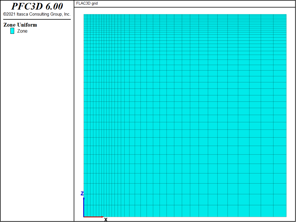
Figure 1: FLAC3D grid.

A uniform mechanical pressure of \(P\) = 1 is applied along the strip location to simulate the strip loading. The fastflow option (zone fluid fastflow on) is selected. The undrained response is calculated first (with model fluid active off and the model stepped to equilibrium). Displacements are then reset to zero, and a coupled fluid-mechanical simulation is performed (using model fluid active on and model mechanical active on) for a period of 8 time units.

The predicted time history of the surface settlement at the center of the strip is compared to the analytical value in Figure 2. The difference between results over the course of the simulation is less than 1%.

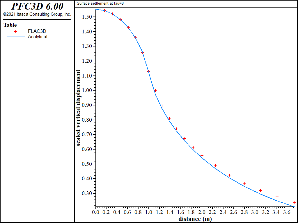
Figure 2: Consolidation settlement (\({\hat{u}-\hat{u}_{und}}\)) at the center of the strip versus log(\(\tau\)) — comparison between FLAC3D and analytical solutions.

The surface consolidation settlement calculated by FLAC3D at the end of the simulation (\(\tau\) = 8) is compared to the analytical solution in Figure 3. The results are in good agreement. The discrepancy observed away from the strip location is attributed to boundary effects. This discrepancy can be reduced by increasing the model lateral and vertical extents.

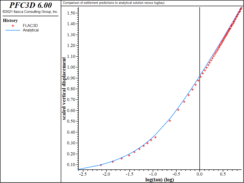
Figure 3: Surface settlement profile at \(\tau\) = 8 — comparison between FLAC3D and analytical solutions.

The predicted excess pore pressure at \(\hat{x}\) = 0, \(\hat{y}\) = 0, \(\hat{z}\) = 9.5, scaled by the undrained pore pressure value, is plotted versus log(\(\tau\)) in Figure 4. The FLAC3D results are compared to the reference solution obtained by Schiffman et al. (1969) and reported by Burghinoli et al. (2001).

An interesting observation is that pore pressure rises initially above the initial undrained value before decaying to zero. This behavior is typical of the Mandel-Cryer effect (Cryer 1963). The peak pressure is slightly underestimated by the FLAC3D solution, but a fair agreement is obtained at later times.

Displacement contours at \(\tau\) = 8 are shown in Figure 5.

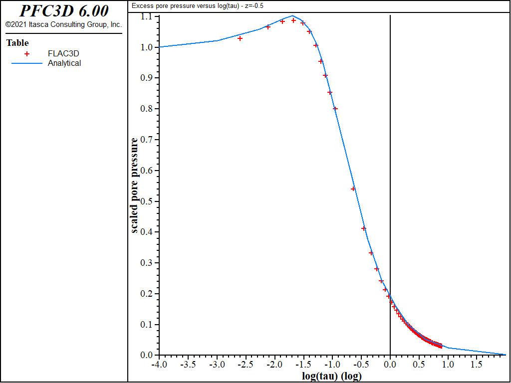
Figure 4: Scaled excess pore pressure at \(\hat{z}\) = -0.5 versus log(\(\tau\)) — comparison between FLAC3D and reference solution given by Schiffman et al. (1969).

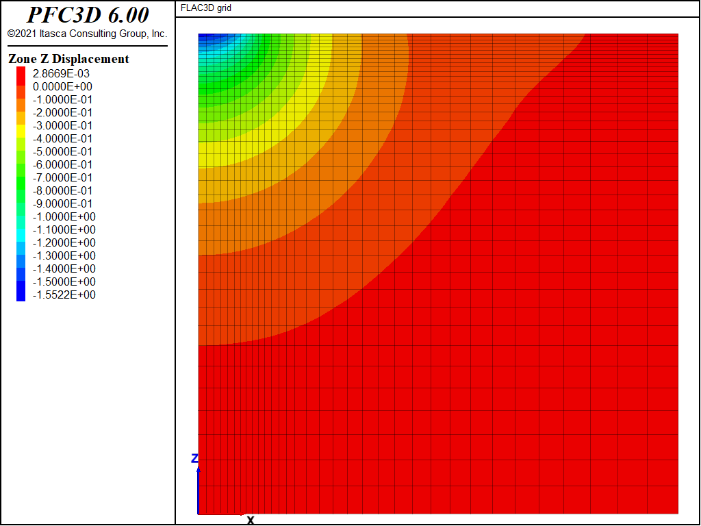
Figure 5: Displacement contours at \(\tau\) = 8.

References

Burghinoli, A., S. Miliziano and F. M. Soccodato. “Effectiveness of the fast-flow algorithm: 2D consolidation benchmark and tunneling application,” FLAC and Numerical Modeling in Geomechanics — 2001 (Proceedings of the 2nd International FLAC Symposium, Lyon, France, October 29 - 31, 2001), pp. 345 - 352. D. Billaux et al., eds. Swets & Zeitlinger (2001).

Cryer, C. W. “A Comparison of the Three-Dimensional Consolidation Theories of Biot and Terzaghi,” Quart. J. Mech. and Appl. Math., XVI, 4, 401-412 (1963).

McNamee, J., and R. E. Gibson. “Plane strain and axially symmetric problems of the consolidation of a semi-infinite clay stratum,” Quart. J. Mech. and Appl. Math. XIII, Pt. 2, (1960).

Schiffman, R. L., A. Chen and J. C. Jordan. “An Analysis of Consolidation Theories,” J. Soil Mech. and Found. Div., ASCE, 95(SM1), 285-312 (1969).

Data File

ConsolidationSettlement.f3dat

model new
model largestrain off
fish automatic-create off
model title "Strip load on semi-infinite elastic medium"
model configure fluid
call 'geometry'
zone generate from-building-blocks
zone face skin
zone gridpoint group 'output' range position (0,0,10) (4,0,10)
call 'fishFunctions'
;@setup
; --- mechanical model ---
zone cmodel assign elastic
zone property bulk=[1.0/3.0] shear=0.5
; --- boundary conditions ---
zone face apply velocity-x 0     range group 'West'
zone face apply velocity-z 0     range group 'Bottom'
zone face apply velocity-y 0     range group 'North' or 'South'
zone face apply velocity (0,0,0) range group 'East'
; --- apply load slowly ---
fish define ramp
    ramp = math.min(1.0,float(global.step)/1000.0)
end
zone face apply stress-normal = -1.0 fish @ramp range position-x 0 1 group 'Top'
; --- fluid flow model ---
zone fluid cmodel assign isotropic
zone fluid property permeability=1.0 porosity 0.3
; --- pore pressure fixed at zero at the surface ---
zone face apply pore-pressure 0 range group 'Top'
; --- settings ---
zone fluid fastflow on
model fluid active off
model step 0
; --- undrained response ---
model solve ratio-local 1e-5
model save 'undrained'
; --- consolidation settlement ---
zone gridpoint initialize displacement (0,0,0)
model fluid active on 
model mechanical active on
model mechanical substep 100 
model mechanical slave on
model fluid substep 10
model step 0
;
[global gpnt0  = gp.near(0,0,10)]
[global gpnt1  = gp.near(0,0,9.5)]
[global u0     = gp.pp(gpnt1)]
fish define zd0
    zd0  = gp.disp.z(gpnt0)
    global uu0  = gp.pp(gpnt1) / u0
    global tau = zone.fluid.time.total*1.0 ; <-- cv = 1.0
    global cons = ana(0,tau,0.5) ; <-- sh = 0.5
end
fish history @zd0
fish history @cons
fish history @uu0
fish history @tau
;
model fluid timestep fix 1e-4
history interval 50
model solve fluid time-total 0.1 or mechanical ratio 1e-5 ; t = 0.1
model fluid timestep auto
history interval 20
model solve fluid time-total 8.0 or mechanical ratio 1e-5 ; t = 8.0
; --- settlement ---
fish define css
    loop foreach local pnt gp.list
        if gp.group(pnt) = 'output' then
            local x = gp.pos.x(pnt)
            table(1,x)  = ana(x,tau,0.5)
            table(11,x) = -gp.disp.z(pnt)
        endif
    endloop
end
@css
; --- pressure ---
history export 3 vs 4 table 40
call 'u-nu0p0.dat'  ; table 50
model save 'strip8'
return