Fragmentation Analysis during a Uniaxial Compression with Crack Tracking Using Fractures

	Example Resources
Data Files	Project: Open “Fragment.p3prj”[1] in PFC3D

Problem Statement

A simple bonded assembly is generated, then brought to failure under uniaxial, unconfined compression. The purpose of this example is to illustrate how fragmentation may be tracked using built-in PFC tools, not to detail the process of building a bonded assembly. For the latter, please refer to the tutorial “Generating a Bonded Assembly” and to the material-modeling support package.

PFC3D Model

A PFC3D bonded assembly is first generated using an approach similar to the one detailed in the “Generating a Bonded Assembly” section. The initial state before compression is shown in Figure 1. In this view, the contacts are colored by the value of the property pb_state (a value of 3 means that parallel bonds are installed) and translated for convenience.

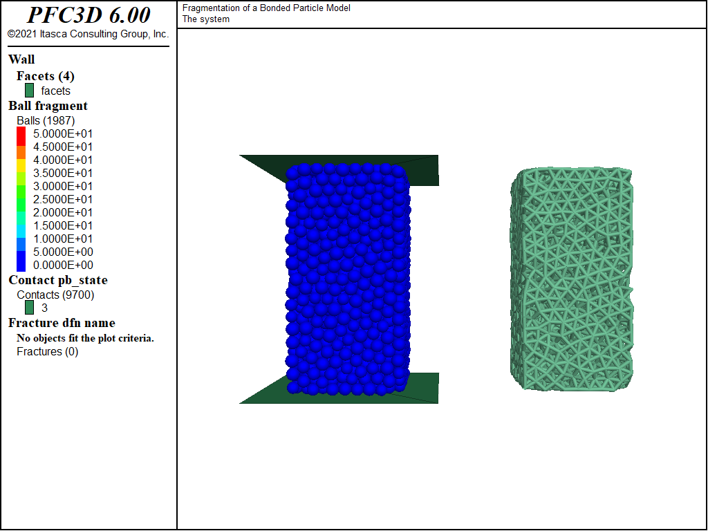
Figure 1: The initial state. Contacts colored by pb_state are translated for convenience.

To perform uniaxial compression, the assembly is confined between top and bottom wall platens (which are assigned equal and opposite velocities along the z-direction), and the model is cycled to a target age limit. The magnitude of the forces exerted by the specimen on the platens is monitored via two histories as a measure of the compressive stress applied to the specimen.

The compression is performed three times with different settings.

• CASE 0 corresponds to a regular run.
• For CASE 1, the fragment logic is activated and the ball results command is used to save partial state information every 0.1 [time-unit] during the course of the simulation.
• For CASE 2, in addition to the use of the fragment logic and the ball results command, a FISH function is registered with the linear parallel bond bond_break callback event, which monitors bond breakage events and creates fractures using the Discrete Fracture Network logic to store their location, size, and orientation. Additionally, the fragments are computed only if a bond breakage event occurred, and ball result states are stored only if the number of fragments in the system changed. The FISH functions used to set up this crack-tracking environment are implemented in “fracture.p3fis”.

Model Results

All three cases produce the same results. The final state for CASE 2 is shown in Figure 2, where contacts and fractures are translated to the right-hand side for convenience. A combination of tensile and shear failures occurred in selected bonded contacts and resulted in the macroscopic failure of the specimen. Forces applied on the platens are identical in magnitude, as shown in Figure 3, and demonstrate the brittleness of the specimen.

Figure 2: State of the system after loading (CASE 3). Right: balls (colored by fragment index). Left: contacts (colored by pb_state) and fractures (colored by shear/tension failure modes) translated for convenience.

Figure 3: Forces (magnitude) measured on the platens vs. time.

The ability to color the balls by their fragment index is a result of the activation of the fragment logic. This logic embeds additional utilities (please refer to the “Fragment” section for a detailed description). For instance, Figure 4 shows the evolution of the volume of the largest fragment (which consists of the whole assembly at the initial state) relative to its initial value, monitored during the course of the simulation.

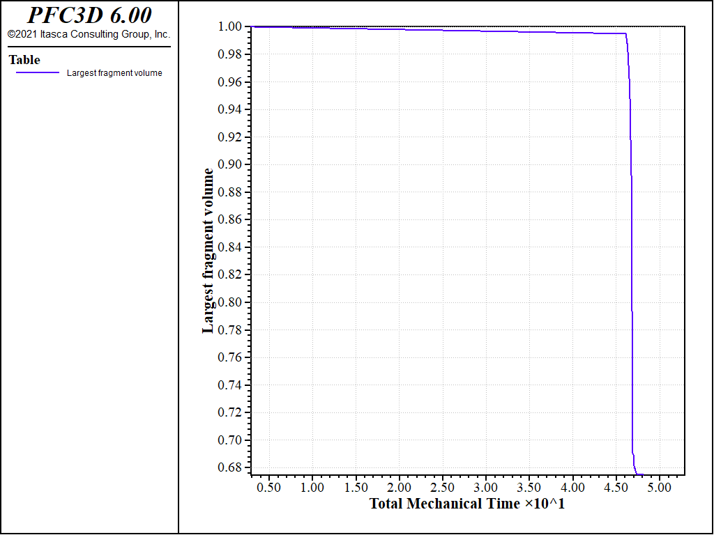
Figure 4: Evolution of the largest fragment volume relative to its initial value.

For CASE 2 and CASE 3, ball configurations and fragment indexes have been saved intermittently during the course of the simulation. Animations can therefore be created using the FISH functions make_movie_case1 (for CASE 1) and make_movie_case2 (for CASE 2). This is an illustration of how the fragment logic and the ball results command can be used together to allow in-depth analysis of the results. Note, however, the costs in terms of memory usage of these two utilities: the sizes of the final model state (SAV) files for CASE 1 and CASE 2 are larger than for CASE 0 (more than 10 times larger for CASE 1). Using custom functions to store model results as performed in CASE 2 can save memory; alternatively, result configurations can be saved as binary files (instead of being stored in RAM) to maintain the memory-usage of the model at a reasonable level.

Conclusion

This example illustrates the steps that may be taken in order to perform a uniaxial compression test on a bonded-particle model with PFC. Moreover, this example describes how the Fragment and Discrete Fracture Network logic can be used, in combination with the ball results command, to track fragmentation and intermittently store pertinent information during the course of the simulation for reuse in a later post-processing step.

Endnote

[1]

This file may be found in PFC3D under the “example_applications/fragments” folder in the Examples dialog (Help —> Examples on the menu). If this entry does not appear, please copy the application data to a new directory. (Use the menu commands Tools —> Copy App Data …. See the “Copy Application Data” section for details.)