Rock Testing

	Example Resources
Data Files	Project: Open “rock_testing.p3prj”[1] in PFC3D

Introduction

This example demonstrates how to simulate laboratory testing of rock core samples; specifically an unconfined compression test and a direct tension test. In the laboratory, a direct tension test is difficult to perform, but in the idealized world of numerical models, this test is possible and provides a more reliable estimate of rock tensile strength than the indirect Brazilian test.

Two different models are compared: a sample bonded with linear parallel bonds and a sample that uses the flat joint contact model. It is well known that parallel bonded models in PFC produce unrealistically low ratios of compressive to tensile strength [Potyondy2004]. This problem can be overcome by using the flat joint contact model in which the contacts have a finite length and therefore particle rotations are resisted [Potyondy2012].

PFC2D Model

Unbonded Sample

First an unbonded assembly with the Linear model assigned to all contacts is created following a similar procedure as in the tutorial “Generating a Bonded Assembly.” The sample is 10 cm long and 5 cm in diameter, conforming to typical laboratory core samples. The walls are created such that they extend past the edge of the sample to allow for changes in the sample size during loading (see {“make_sample.p2dat” in 2D; “make_sample.p3dat” in 3D}).

The contact stiffnesses are set using contact methods instead of properties. The contact methods perform small calculations to automatically set the properties. So, for example, in 3D, the normal stiffness at a contact is proportional to the effective Young’s modulus and the particle radius as described here. We can therefore set the contact deformability property ‘emod’ (in stress units) and the linear stiffnesses will automatically be calculated based on the particle radii. In this example, it is assumed that stress quantities are in Pa. The unbonded sample is shown below.

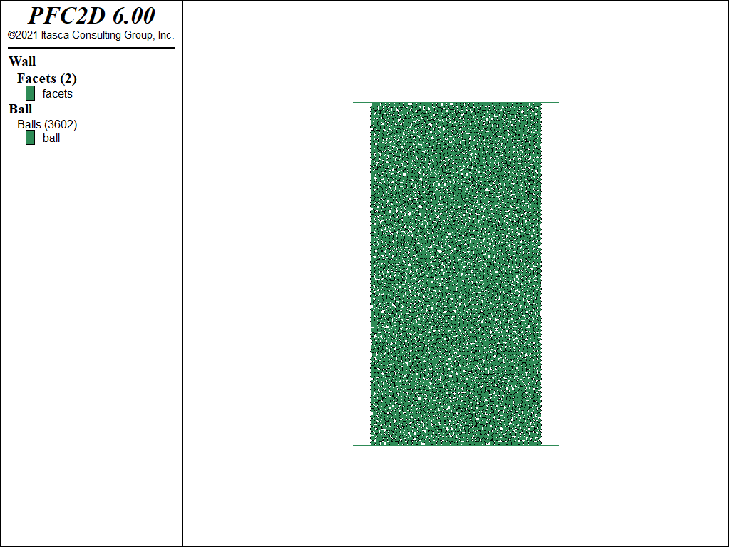
Figure 1: Unbonded material model.

The parallel bonded sample is created using the commands in {“parallel_bonded.p2dat” in 2D; “parallel_bonded.p3dat” in 3D}. The parallel bond stiffnesses are again set using methods. Be careful with parallel bonds in that both the linear stiffness (contact method deform) and the bond material stiffness (contact method pb_deform) are set.

; set linear stiffness
contact method deform emod 1.0e9 krat 1.0

; set stiffness of bond material
contact method pb_deform emod 1.0e9 krat 1.0

When the contact type is changed from linear to parallel bond, the linear stiffnesses are not inherited and must be set again.

One other thing to note is the use of lin-mode 1

; Set the linear force to 0.0 and force a reset of the linear contact forces. 
contact property lin_force 0.0 0.0 lin_mode 1
ball attribute force-contact multiply 0.0 moment-contact multiply 0.0 

when resetting the linear forces to 0. This ensures that contact normal forces will be generated based on relative displacements (incrementally), rather than absolute overlaps between entities.

Unconfined Compressive Strength

A UCS test is performed by simply moving the top wall downward and the bottom wall upward as shown in the file {“ucs.p2dat” in 2D; “ucs.p3dat” in 3D}. The only trick is recording the axial stress and strain. A small FISH function is used to sum all of the vertical forces acting on the walls and then dividing by the sample width to get the axial stress. The strain is simply calculated from the wall displacement divided by the initial sample length. The initial sample width and length are determined at the start of the test. Note that this will introduce a small error in the stress calculation because the sample width will actually change during the test and this is not accounted for in the function.

A set of FISH functions that are very useful when simulating rock tests are given in {“fracture.p2fis” in 2D; “fracture.p3fis” in 3D}. These functions track bond breakages, and for each bond breakage, a fracture is added to a DFN. The cracks can then be easily plotted during and/or after the test. In addition, the functions delineate fragments in the sample. A fragment is a piece of the model that is not connected to any other pieces with intact bonds.

The sample is loaded until the axial stress falls below 70% of the peak stress. The result of the UCS test on the parallel bonded sample is shown in the next figure and the axial stress versus the axial strain plotted on top of the sample. The stress and strain are calculated assuming compressive stress is negative, but in the next figure, the plot is reversed to show compression positive in keeping with rock mechanics conventions. The UCS for this sample is 33.9 MPa. Note that running this example on different computers may produce slightly different results due to the randomness inherent in the particle packing.

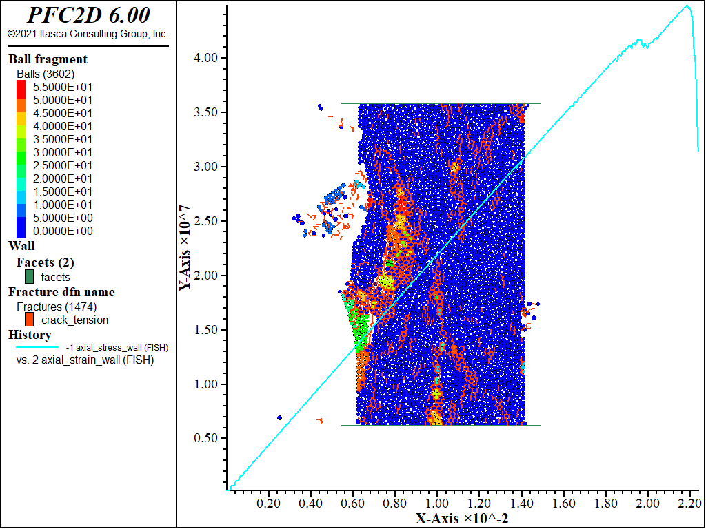
Figure 2: Parallel bonded material after the UCS test. Cracks are shown in black and red lines indicating tensile and shear failure, respectively. Axial stress vs. axial strain (positive compression) is plotted as a green line.

Direct Tension Test

A direct tension test is simulated on the same numerical sample as was used in the UCS test (see {“tension.p2dat” in 2D; “tension.p3dat” in 3D}). To perform the test, the walls are deleted and a row of particles at the top and bottom of the sample are identified as “grips” (figure below). The top grip is moved upward and the bottom grip downward to apply tensile loading.

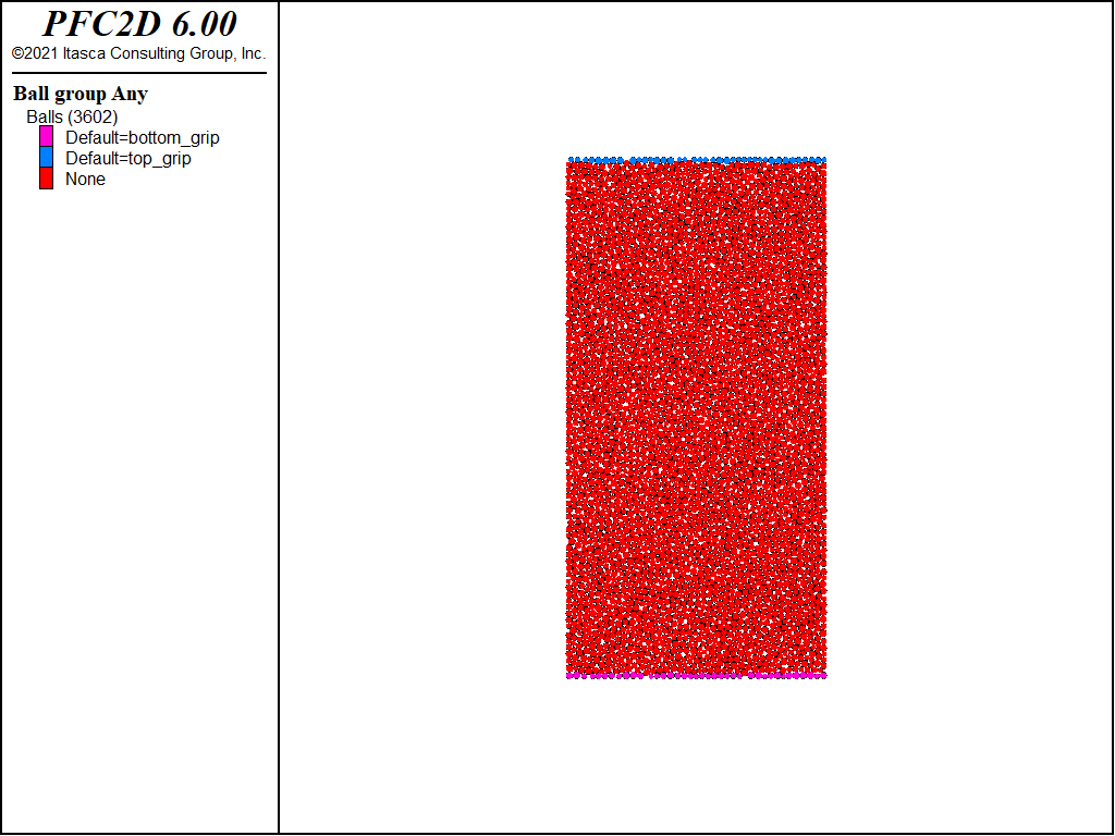
Figure 3: Particle grips used to apply tensile loading are shown in green and red.

Since the walls have been deleted, the stress and strain must be measured in a different way. Stress is measured by creating a single measurement circle in the center of the sample. The stress is computed by averaging the contact forces within the circle as described here.

The strain is computed by observing the displacement of two gage particles. A particle at the top of the model and another at the bottom. The relative displacement of the two gage particles divided by the initial distance between them gives the axial strain.

As with the UCS test, the model is loaded until the axial stress is 70% of the peak. The stress-strain response is shown in Figure 4 with the final sample configuration. Remember we are assuming compression positive, so the tensile strength is the most negative value in the plot. The peak tensile stress is 6.8 MPa. This yields a ratio of compressive to tensile strength of ≈5, considerably lower than the expected value of 10–20.

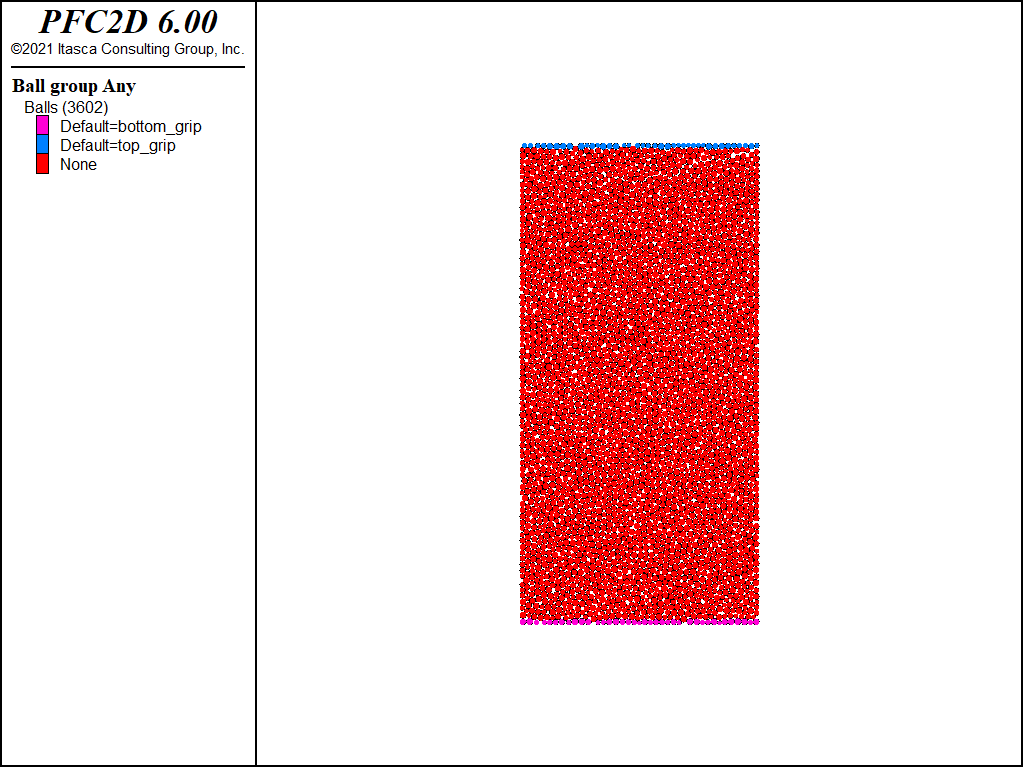
Figure 4: Parallel bonded material after the direct tension test plotted with axial stress versus axial strain (compression positive).

Flat-Joint Contact Model

It is well known that the parallel bonded model yields unrealistically low ratios of compressive to tensile strength and unrealistically low friction angles for rock [Potyondy2004]. A likely reason for this is that round particles are used to simulate angular grains. There is not enough resistance to rotation, especially after bonds have broken. The flat-joint contact model overcomes this deficiency by simulating a contact as a {flat line in 2D; disk in 3D} composed of many subcontacts such that rotation is resisted (see the “Flat-Joint Model” section for a detailed description).

The UCS and direct tension tests were repeated with a flat-jointed material (shown in {“flat_joint.p2dat” in 2D; “flat_joint.p3dat” in 3D}). The same properties were assigned as for the parallel bonded model. Stress-strain curves and failed samples for the two tests are shown in the next two figures. These plots show a peak compressive stress of 70.5 MPa and tensile strength of 7.1 MPa, yielding a ratio of compressive to tensile strength of ≈10.

Interestingly, the tensile strength is almost the same as for the parallel bonded material, but the compressive strength is much higher. The mechanism of tensile failure is approximately the same in both samples; the breaking of a few bonds in tension and rapid propagation of the fracture across the sample. In compression, the failure is much more complicated and involves some combination of axial splitting and shear failure along en-echelon arrays of tensile cracks. The flat-joint model shows many more cracks, but the strength is higher, possibly because the cracks cannot so easily coalesce to cause failure because particle rotations are somewhat suppressed.

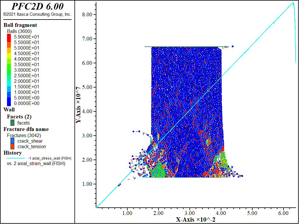
Figure 5: Results of the UCS test on the flat-jointed model.

Figure 6: Results of the direct tension test on the flat-jointed model.

PFC3D Model

The 3D model is essentially the same with a slightly larger ball size. The sample shape in 3D is a cylinder. The final state for the flat-jointed 3D model in the UCS test is shown below.

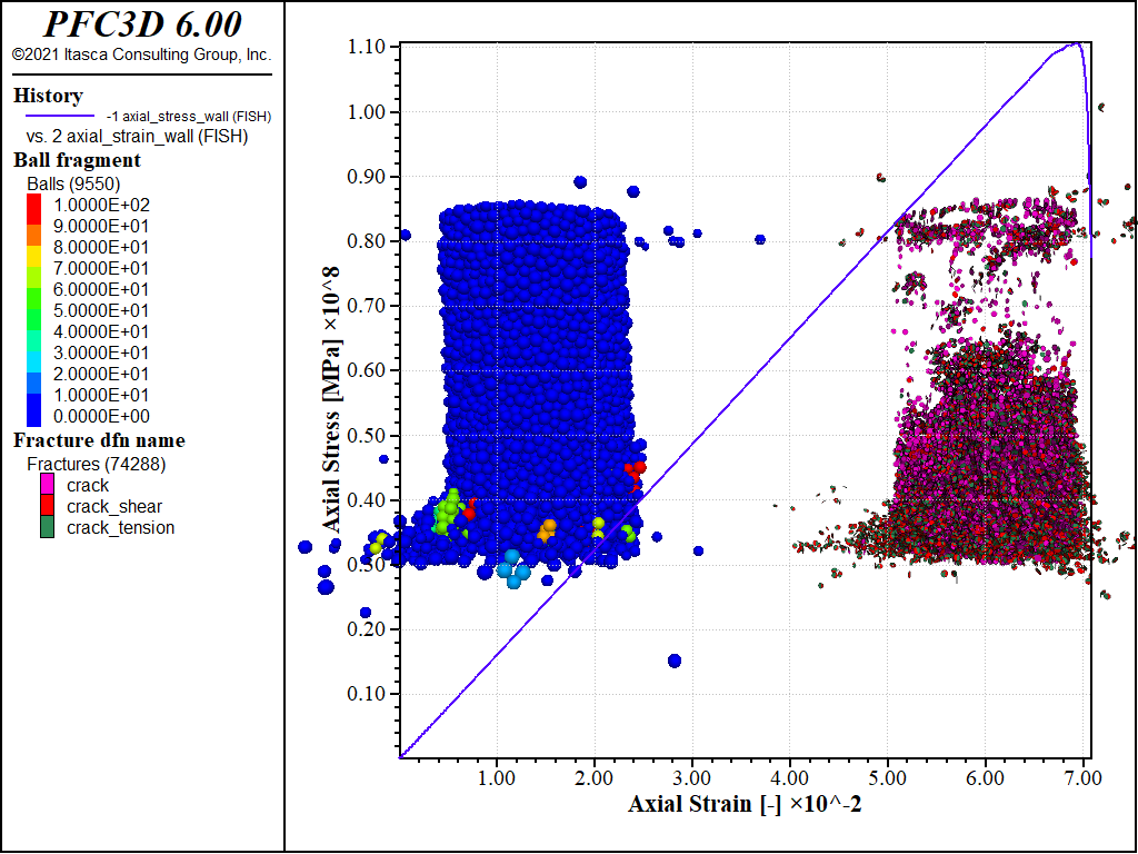
Figure 7: 3D flat-joint model after UCS test.

Discussion

This example shows how to simulate a UCS test and direct tension test and shows how the flat-joint contact model gives a more realistic compressive to tensile strength ratio than the parallel bonded model. This example is really a simplified version of what is provided in the material-modeling support package. This package creates and defines particular instances of parallel-bonded and flat-jointed materials, and also provides crack monitoring as well as facilities to perform standard rock-mechanics tests (including direct-tension and compression) upon these materials.

References

[Potyondy2004]

(1, 2) Potyondy, D. O., and P. A. Cundall. “A Bonded-Particle Model for Rock,” Int. J. Rock Mech. & Min. Sci., 41(8), 1329-1364 (2004).

[Potyondy2012]

Potyondy, D.O. (2012) “A Flat-Jointed Bonded-Particle Material for Hard Rock,” paper ARMA 12-501 in Proceedings of 46th U.S. Rock Mechanics/Geomechanics Symposium, Chicago, USA, 24–27 June 2012.

Endnote

[1]

This file may be found in PFC3D under the “example_applications/rocktest” folder in the Examples dialog (Help —> Examples on the menu). If this entry does not appear, please copy the application data to a new directory. (Use the menu commands Tools —> Copy App Data …. See the -ref–dlg_copyappdata- section for details. [CS: commented out because UI material not present as of 9/25/17, therefore link is broken. Put back in when UI material is restored])