
Slip on a Fault
| Tutorial Resources | |
|---|---|
| Data Files | Project: Open {“joint_slip.p2prj” in PFC2D; “joint_slip.p3prj” in PFC3D} [1] |
Introduction
This tutorial demonstrates how to simulate sliding on a single fault or joint. A fault can exhibit stable (locked) or unstable (sliding) behavior depending on the magnitude of shear and normal stress acting on the fault and the fault friction angle. To test this in PFC, a bonded particle model is created using the linear parallel bond model and a joint is added by applying the smooth joint model to selected contacts. The model is subjected to gravitational loading and the sliding behavior of the joint is examined for different joint friction angles.
PFC2D model
Bonded Assembly
A 6×6 m sample is constructed by following the same procedure as in the tutorial “Generating a Bonded Assembly”. The commands, not detailed herein, are in the data file “make_intact.p2dat”.
The intact material model is shown in Figure 1. The figure is created by plotting balls and coloring by (currently all 0). Contacts are also plotted and colored by the (currently all linear parallel bonds).
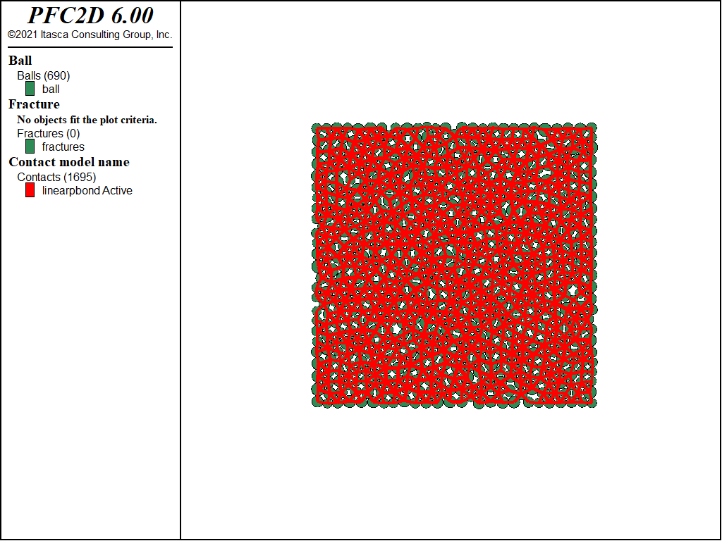
Figure 1: Intact material model.
Adding a Fault
The commands for adding a fault to the model are provided in “make_fault.p2dat”. First the intact model is restored. The easiest way to add faults is to first create a Discrete Fracture Network (DFN). In this example, a DFN is created that contains only a single fracture. The fracture has a dip of 30 degrees and a diameter of 20 m to ensure that it spans the entire model. This can be accomplished with a single command:
fracture create dip 30 size 20.0
By default, the shape of the fracture is a line (disk in 3D), and the coordinates of the center default to 0.0. You can add the DFN to your plot to view it as shown in Figure 2. In this figure, the DFN color was changed to black for ease of viewing. This can be found under the DFN plot Attribute, “Color Opt – Colors – facets”.
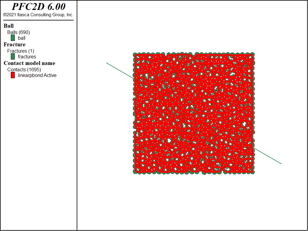
Figure 2: Model with DFN.
The properties of the smooth joint contacts can be set by first assigning properties to the DFN. Whatever properties are assigned to the DFN will automatically be assigned to contacts created with the fracture contact-model model command (see below). The properties for the fault are shown in the following command:
fracture property ...
  'sj_kn' 2e9 'sj_ks' 2e9 'sj_fric' 0.70 'sj_coh' 0.0 'sj_ten' 0.0 'sj_large' 1
The friction angle is set to 35°. Since this is more than the dip of the fault, it is expected that there will be no sliding on the fault. Note that, as input, PFC requires the dimensionless friction coefficient \(\mu\) (tangent of the friction angle) rather than the friction angle in degrees. Setting the sj_large parameter to 1 ensures that the joint contacts behave properly when large strain is expected. Essentially, if two smooth joint contacts move far enough apart, then the contact is removed. Setting sj_large=1 adds a small amount of computational overhead since contacts need to be checked to see if they have moved apart. The smooth joint contact model is then assigned to all contacts that intersect the DFN (in this case, a single fracture). A contact intersects the fracture if one particle centroid is on one side of the fracture and the other particle centroid is on the opposite side. It is possible to specify a wider fault zone using the ‘distance’ keyword. Setting a non-zero value for the distance will pick up extra contacts within the specified distance of the fault. For this example, we specify a distance of 0.1. The command to create smooth contacts along the joint is as shown:
fracture contact-model model 'smoothjoint' install dist 0.1 activate
Your plot should now show the smooth joint contacts and parallel bonded contacts in different colors (Figure 3).
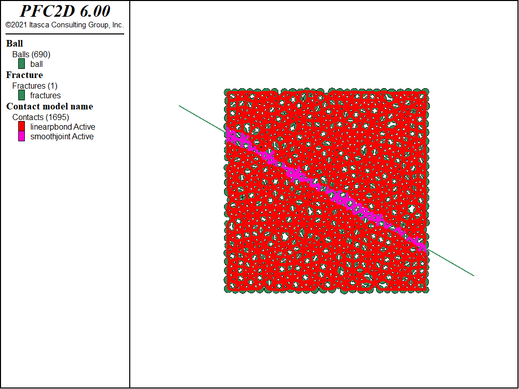
Figure 3: Faulted material.
Smooth joint contacts will usually have an orientation different from the default orientation dictated by the two connecting particles. In general, the orientation of the smooth joint contact is set to be parallel to some fault plane so that slip along this plane may occur without the ‘bumpiness’ that would result if contacts were not reoriented (see link for more information). The orientation of the smooth joint contacts is automatically set to be the same as the orientation of fractures in a DFN. Under the contact plot item attributes, check the box for . This will render the smooth joint contacts with their ‘true’ orientations (Figure 4). Note that in 2D, contacts are shown as lines parallel to the normal force direction (perpendicular to the fault). In 3D, the contacts can be rendered as disks parallel to the shear direction (parallel to the fault), as shown in Figure 8.

Figure 4: Contacts, balls, and DFN for the model with a fault added.
CS: change to commands makes the writeup out of whack here; compare two lines needed originally with PFC 5 are now just one in PFC 6
Finally, we want new contacts that form as the joint is sliding to be assigned the smooth joint contact model as well. This is accomplished by activating the DFN contact model assignment:
fracture contact-model model 'smoothjoint' install dist 0.1 activate
Gravitational Loading
The full data file for this stage is “load.p2dat”. Gravitational loading is applied by first fixing a row of particles at the bottom of the model. Gravity is then turned on and an acceleration of 10 m/s2 is assigned. The default direction for acceleration due to gravity in 2D is in the negative y direction.
; Fix row of balls at the bottom
ball fix vel range position-y -6 -5.5

; Turn on gravity
model gravity 10
If you change the attribute for the balls to , you can see the fixed particles at the bottom (Figure 5).
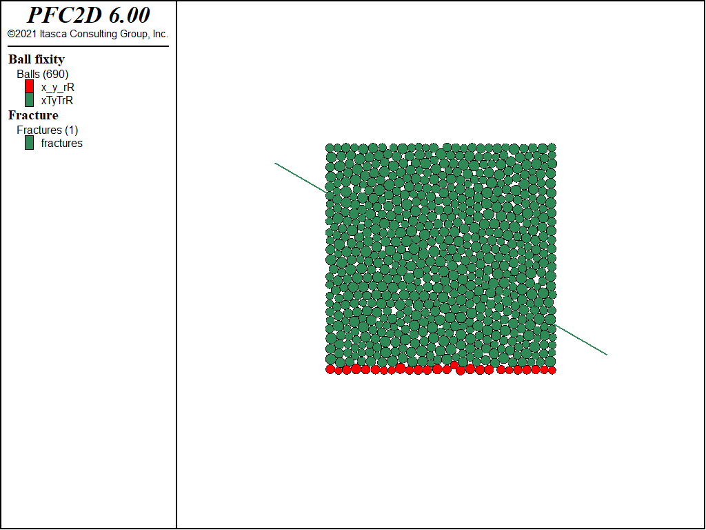
Figure 5: Balls colored by their fixity condition.
Since we expect the model to be stable, we can then just use the solve command to bring it to equilibrium.
model solve ratio-average 1e-5
The particles displace downward with magnitudes as shown in Figure 6.
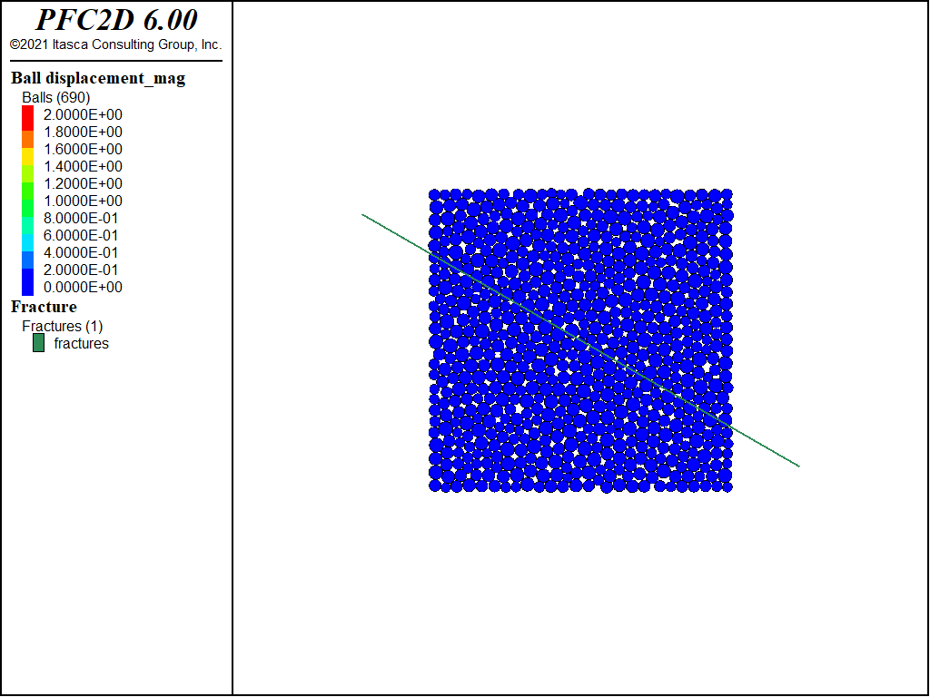
Figure 6: Particle displacements after reaching equilibrium in the model with a fault friction angle of 35°.
Now try setting the fault friction angle to 25° (\(\mu\) = 0.466). The following command will change the friction of all existing and future smooth joint contacts within range of the DFN.
fracture property 'sj_fric' 0.466
Since we are expecting a lot of motion, it is a good idea to decrease the local damping to get more realistic behavior:
ball attribute damp 0.1
Since we expect the model to slide unstably, we cannot use the solve command. Instead we will execute 20,000 cycles:
; Do not use solve command since we expect unstable sliding
model cycle 20000
The plot of ball displacement now clearly shows the sliding on the fault (Figure 7).
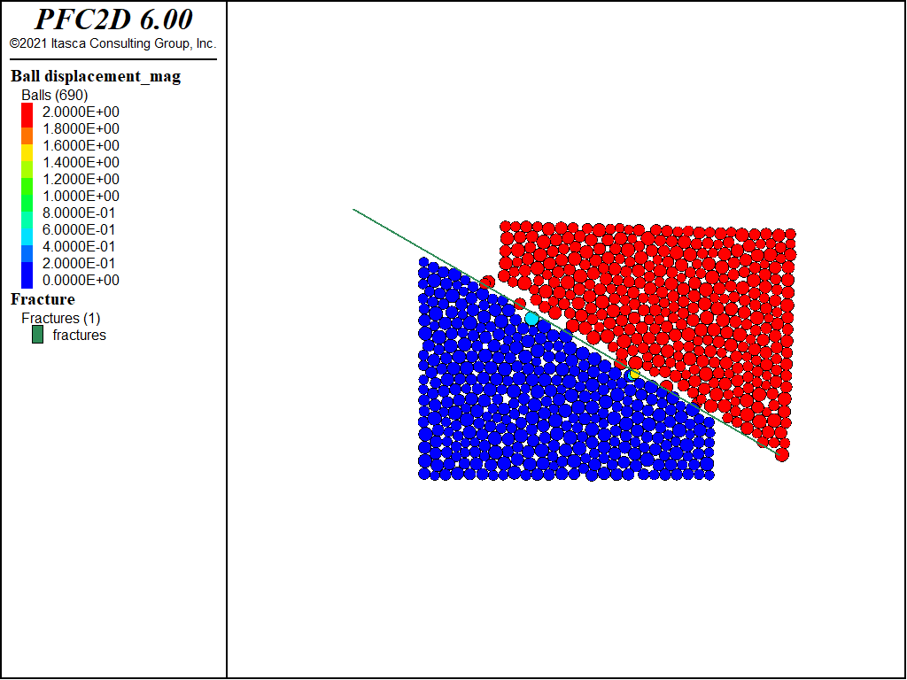
Figure 7: Particle displacements after 20,000 steps in the model with a fault friction angle of 25°.
PFC3D model
The 3D model is essentially the same with a slightly larger ball size. The data files are “make_intact.p3dat”, “make_fault.p3dat”, and “load.p3dat”. The final state for the 3D model is shown in Figure 8.
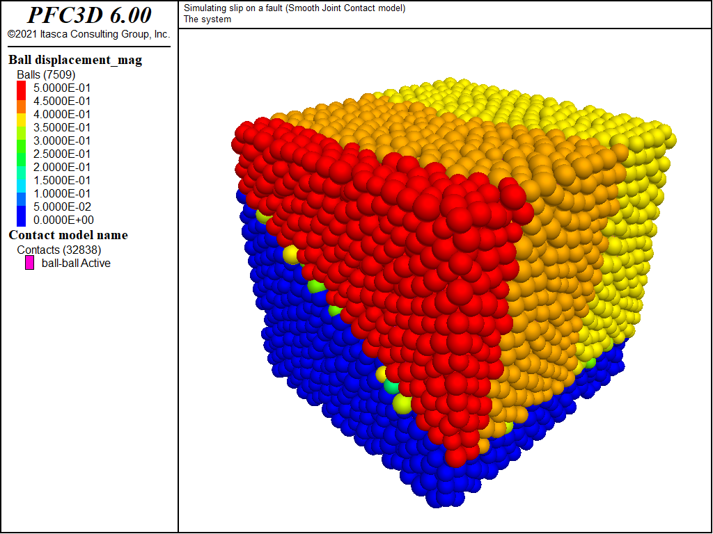
Figure 8: 3D model after slip on fault with friction angle of 25°.
Discussion
This example shows how to simulate sliding on a single fault by assigning the Smooth Joint Contact Model to contacts that intersect a circular fracture. The techniques shown here could also be used to simulate a sample of rock with many intersecting faults; however, in that case, a much higher resolution would be required. By using the fracture contact-model model command, intersecting contacts are automatically identified and assigned the correct orientation and properties. If you wish to simulate multiple fracture sets with different properties, multiple DFNs could be created with different properties assigned to them.
Endnote
| [1] | These may be found in PFC3D under the “tutorials/joint_slip” folder in the Examples dialog ( on the menu). If this entry does not appear, please copy the application data to a new directory. (Use the menu commands . See the Copy Application Data section for details.) |
| Was this helpful? ... | PFC 6.0 © 2019, Itasca | Updated: Nov 19, 2021 |