
Tip-Loaded Cantilever Beam
| Problem Resources | |
|---|---|
| Data Files | Project: Open {“Cantilever.p2prj” in PFC2D; “Cantilever.p3prj” in PFC3D} [1] |
Problem Statement
A tip-loaded cantilever beam is modeled using PFC2D and PFC3D. The computed deformations and the maximum shear and normal stresses are compared with the analytical beam-theory solution. This problem demonstrates the capabilities of the parallel-bond logic in PFC.
The physical model of the beam, with a length of 200 inches and a circular cross-section with radius, \(R\), of 8 inches in 3D, is shown in portion (a) of Fig. 1 below. In 2D, the beam has a rectangular section of unit thickness and height \(2R\). The beam material is 2024-T3 aluminum with a Young’s modulus, \(E\), of 1 × 10⁴ ksi and a shear modulus, \(G\), of 3759.4 ksi. The loading consists of transverse load, \(F\), axial load, \(P\), (in-plane) bending moment, \(M\), and (out-of-plane) twisting moment, \(T\) (in 3D only), applied at the beam tip.
Closed-Form Solution
A closed-form expression for the deformation and maximum shear and normal stresses of the cantilever beam is given by simple beam theory. The solution is expressed in terms of the Cartesian coordinate system shown in Fig. 1 below. The origin of this coordinate system is at the fixed end of the beam, and the \(x\)-axis is directed toward the beam tip and lies along the neutral axis.
Transverse load, \(F\), and bending moment, \(M\), produce a transverse deflection, \(Δ_z\), and a rotation about the \(y\)-axis, \(θ_y\). Axial load, \(P\), produces an axial extension, \(Δ_x\). The twisting moment, \(T\), produces a rotation, \(θ_y\), about the \(x\)-axis. These deformations are given by McGuire and Gallagher (1979):
where:
The total contribution from the bending load and applied twisting moment to the maximum shear and normal stresses is given by
The extension of the beam subjected to an axial load, \(P\), can be found using \(P/K\), where \(K\) is the equivalent stiffness of a single spring. If the beam is modeled by a collection of \(n\) springs, each with a stiffness of \(k^{(i)}\), \(K\) can be determined based on whether the collection of springs is acting in series or in parallel, and is given by
For the special case in which all of the springs have the same stiffness, \(k\), the expression for the equivalent stiffness simplifies to
The analytical solution for the beam modeled using \(n\) parallel bonds and \(n\) contacts is found by noting that the parallel bonds act in parallel with the contact springs to carry the load, and that the equivalent stiffnesses of the parallel bonds and the ball contacts are given by Equation (5), such that the equivalent stiffness of the entire beam is given by
where \(\bar k_n\) and \(k_n\) are the normal stiffnesses of each parallel bond and each ball, respectively. Note that the contact stiffness for two balls with identical stiffnesses is equal to half the ball stiffness.
Numerical Model
The cantilever beam is modeled in PFC by joining together a row of 11 balls of equal radius with parallel bonds, as shown in portion (b) of Fig. 1 below. The ball radii are chosen to be larger than the radius of the cantilever beam in order to demonstrate the relation between each parallel bond and an equivalent elastic cylinder. The radius of each ball is 10 inches, but the radius of each parallel bond is set to 8 inches to match the physical beam. The normal and shear stiffnesses of the parallel bonds are chosen such that the collection of ten equivalent elastic cylinders, shown in portion (c) of Fig. 1 below, mimics the physical beam. Thus, the chosen values are
Both the normal and shear strength of the parallel bonds are set to the large value of 1 × 10⁵ ksi, so that inertial effects arising from sudden application of the loads do not cause the parallel bonds to break. The normal and shear stiffnesses of each of the balls (2.0106 × 10⁵ kips/inch) are chosen by setting the second term of Equation (6) equal to the overall beam stiffness of \(AE/L\).
The velocities of all six degrees of freedom are fixed to zero for the ball at the origin of the coordinate system, and three of the generalized forces are applied to the ball at the opposite end of the assembly. The model is then cycled until static equilibrium is reached (i.e., the velocities of all balls become negligible). Since the closed-form solution based on simple beam theory is no longer valid when an axial load is applied to the deflected configuration, because the problem becomes geometrically nonlinear, the axial load is applied as a separate case.
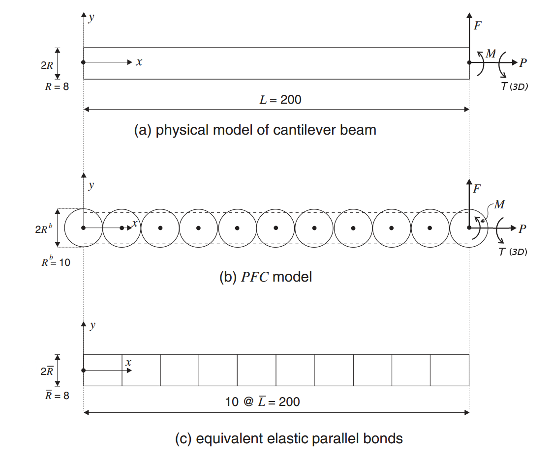
Figure 1: Cantilever beam and PFC model. (\(M\) is an in-plane bending moment. \(T\) is an out-of-plane twisting moment in the 3D model.)
Results and Discussion
PFC3D Model
The deformations at the tip of the beam arising from the application of transverse load, \(F\), of 1.0 kip; bending moment, \(M\), of 100.0 kip × inch; and twisting moment, \(T\), of 2000.0 kip × inch are compared with the closed-form solution in Table 2. The total rotation of the ball at the beam tip is monitored by activating orientation tracking (using the model orientation-tracking command). FISH variables _xdel11, _ydel11 and _xrot11, _zrot11 store accumulated displacements and rotations, respectively, at the beam tip. The computed values of maximum normal and shear stress within the parallel bonds are found by using the FISH function get_maxpbstr. The maximum normal stress is found to be acting in the parallel bond centered at \(x\) = 10. The value of 7.2117 × 10⁻¹ ksi agrees exactly (within five significant figures) with the analytical solution of 7.2117 × 10⁻¹ ksi, at \(x\) = 10. The maximum shear stress arises from the transverse load and the twisting moment and is uniform throughout the length of the beam. The value of 2.4918 ksi agrees exactly (within five significant figures) with the analytical solution. These results can be obtained by printing _maxpbnstr, _maxpbsstr, _maxpbnx, and _maxpbsx.
| Numerical | Analytical | Relative Error | |
|---|---|---|---|
| \(\Delta_y(L)\) | 1.4512 × 10⁻¹ in. | 1.4506 × 10⁻¹ in. | < 0.1% |
| \(\theta_z(L)\) | 1.2436 × 10⁻³ rad. | 1.4506 × 10⁻³ rad. | < 0.1% |
| \(\theta_x(L)\) | 1.6535 × 10⁻² rad. | 1.6537 × 10⁻² rad. | < 0.1% |
The results of three separate cases in which only the axial load, \(P\), was applied to the beam are presented here. The cases differ based on whether the load is carried by the parallel bonds, the contact springs, or both.
In the first case, \(P\) = +1000 kips, and the parallel bonds are left intact. This puts the beam in tension, and all of the load is carried by the parallel-bond springs. The computed axial extension of 9.9472 x 10⁻² agrees exactly (within five significant figures) with the analytical solution.
In the second case, \(P\) = -1000 kips, and the parallel bonds are removed. This puts the beam in compression, and the load is carried by the contact springs between the balls. The computed axial extension of -9.9473 × 10⁻² is within 0.1 percent of the analytical solution of -9.9472 × 10⁻².
In the third case, \(P\) = -1000 kips, and the parallel bonds are left intact. This puts the beam in compression, and the load is shared by both the parallel bond springs and the contact springs between the balls. This case does not correspond to the physical problem, since both the parallel bond and contact stiffnesses were chosen assuming that only one was acting at a time. The analytical solution for this case is found using Equation (6). The computed axial extension of -4.9736 × 10⁻² agrees exactly (within five significant figures) with the analytical solution.
PFC2D
The deformations at the tip of the beam arising from the application of transverse load, \(F\), of 1.0 kip, and bending moment, \(M\), of 100.0 kip × inch, are compared with the closed-form solution in Table 3. The total rotation of the ball at the beam tip is monitored by activating orientation tracking (using the model orientation-tracking command). FISH variables _xdel11, _ydel11, and _rot11 store accumulated displacements and rotations, respectively, at the beam tip. The computed values of maximum normal and shear stress within the parallel bonds is found by using the FISH function get_maxpbstr. The maximum normal stress is found to be acting in the parallel bond centered at \(x\) = 10. The value of 7.2117 × 10⁻¹ ksi agrees exactly (within five significant figures) with the analytical solution of 7.2117 × 10⁻¹ ksi, at \(x\) = 10. The maximum shear stress arises from the transverse load and the twisting moment and is uniform throughout the length of the beam. The value of 2.4918 ksi agrees exactly (within five significant figures) with the analytical solution. These results can be obtained by printing _maxpbnstr, _maxpbsstr, _maxpbnx, and _maxpbsx.
| Numerical | Analytical | Relative Error | |
|---|---|---|---|
| \(\Delta_y(L)\) | 1.3685 in. | 1.3672 in. | < 0.1% |
| \(\theta_z(L)\) | 1.1718 × 10⁻² rad. | 1.1719 × 10⁻² rad. | < 0.1% |
The results of three separate cases in which only the axial load, \(P\), was applied to the beam are presented here. The cases differ based on whether the load is carried by the parallel bonds, the contact springs, or both.
In the first case, \(P\) = +1000 kips, and the parallel bonds are left intact. This puts the beam in tension, and all of the load is carried by the parallel-bond springs. The computed axial extension of 1.2499 agrees exactly, within four significant figures, with the analytical solution of 1.25.
In the second case, \(P\) = -1000 kips, and the parallel bonds are removed. This puts the beam in compression, and the load is carried by the contact springs between the balls. The computed axial extension of -1.2499 agrees exactly, within four significant figures, with the analytical solution of -1.25.
In the third case, \(P\) = -1000 kips, and the parallel bonds are left intact. This puts the beam in compression, and the load is shared by both the parallel bond springs and the contact springs between the balls. This case does not correspond to the physical problem, since both the parallel bond and contact stiffnesses were chosen assuming that only one was acting at a time. The analytical solution for this case is found using Equation (6). The computed axial extension of -6.2497 × 10⁻¹ agrees exactly (within four significant figures) with the analytical solution of -6.25e-1.
References
McGuire, W., and R. H. Gallagher. Matrix Structural Analysis, p. 87. New York: John Wiley & Sons, 1979.
Endnote
| [1] | This file may be found in PFC3D under the “verification_problems/Cantilever” folder in the Examples dialog ( on the menu). If this entry does not appear, please copy the application data to a new directory. (Use the menu commands . See the “Copy Application Data” section for details.) |
⇐ Data File for “Strength of a Face-Centered Cubic Array of Spheres”
Problem |
Data Files for “Tip-Loaded Cantilever Beam” Problem ⇒
| Was this helpful? ... | PFC 6.0 © 2019, Itasca | Updated: Nov 19, 2021 |