Measure Logic

	Problem Resources
Data Files	Project: Open {“MeasureLogic.p2prj” in PFC2D; “MeasureLogic.p3prj” in PFC3D} [1]

Problem Statement

The measure logic (see the measure create command) is exercised with PFC to compute porosity. Two regular packings composed of mono-sized balls organized in crystal-like patterns and a polydisperse packing are generated. The porosity is computed using measurement circles (or spheres in 3D) with different radii. The accuracy of the numerical results is evaluated through comparison to analytical values.

Closed Form solution

Two crystal-like packings are considered. Both packings consist of equal-radius balls in contact with no overlap. The first packing is a simple cubic arrangement (see Fig. 1 for a 2D view) in which each ball is in contact with four neighbors in 2D (six in 3D). The second packing is a hexagonal arrangement (see Fig. 2) in which each ball is in contact with six neighbors in 2D (twelve in 3D). The hexagonal arrangement is the closest of all possible regular two-dimensional or three-dimensional packings. For both packings, the porosity is independent of the size of the balls, provided that the packing is extended over a very large region so that the effect of boundaries is negligible (Refer to [Deresiewicz1958a] for a thorough discussion of packings in both two and three dimensions).

The density, \(D\), of a packing is defined as the ratio of the area of space occupied by solid matter, \(A_s\), to the total area, \(A\). If we assume that the total area comprises both solid and void areas and that there is no overlap, then the density is related to the porosity, \(n\), by the relation

\[n = 1 - D = 1 - \frac{A_s}{A}\]

For the simple cubic packing, we have, in two dimensions:

(1)\[n = 1 - \frac{\pi R^2}{(2R)^2}=1-\frac{\pi}{4} \approx 0.2146\]

and, in three dimensions:

(2)\[n = 1 - \frac{4/3 \pi R^3}{(2R)^3}=1-\frac{\pi}{6} \approx 0.4764\]

For the hexagonal packing, in two dimensions, we have:

(3)\[n = 1 - \frac{\pi R^2}{(\sqrt{3}R)(2R)}=1-\frac{\pi}{2 \sqrt{3}} \approx 0.0931\]

and, in three dimensions:

(4)\[n = 1 - \frac{8 \pi R^3}{(6\sqrt{3}R^2)(4R\sqrt{2/3})}=1-\frac{\pi}{3 \sqrt{2}} \approx 0.2595\]

In the case of a polydisperse assembly, a specific procedure is implemented to compute the porosity (see the get_poros function in “PolydisperseAssembly.p2dat” and “PolydisperseAssembly.p3dat”) using the ratio between the sum of the surface (volume in 3D) of each ball in the model over the total surface (volume in 3D) of the sample.

(5)\[n = 1-\frac{S_{balls}}{S} \quad (2D) \quad \quad n = 1-\frac{V_{balls}}{V} \quad (3D)\]

Numerical Model

Several parameterized FISH functions are used to generate the measurement circles (spheres in 3D) that will be used to compute the porosity of the packings.

These functions are defined in {“MeasureLogic.p2dat” for 2D; “MeasureLogic.p3dat” for 3D}.

The function define_meas_parameters takes two arguments: nmeas, whereby the user can define the number of measurement regions to be created within the packing; and pcntg, through which the tolerance value can be defined in the measure create command. This last parameter determines the error (< pcntg) tolerance accepted during porosity computation in the measurement regions. See the reference page for details.

The measurement regions have random size and random position in the model. This is defined in the create_meas_regions function.

To verify the accuracy of the porosity computation, a check_error function with three arguments is defined: val, the reference value of the porosity, which is computed through Equations (1), (2), (3), (4) in the case of the regular assemblies, or directly using Equation (5) in the case of the polydisperse assembly, to be compared to the numeric results; t, a string variable which allows definition of the name of the table that will contain the values of the errors committed in the porosity measurement; and average_radius, the average radius of the balls comprising the assembly which will be used to normalize the diameters of the measurement regions while post-processing the results of the simulation.

In the case of the regular assemblies, a parameterized FISH function is used to construct each packing using the ball generate command in {“RegularAssembly.p2dat” for 2D; “RegularAssembly.p3dat” for 3D}. This function has three arguments: size, resolution, and packing type (size, nres, itype). Two models are built for each packing. These models contain 9 rows and 9 columns of balls (9x9x9 in 3D) and 30 rows and columns (30x30x30 in 3D), respectively.

A screenshot of the cubic and hexagonal arrangements (9x9 packings, low resolution, 2D view) is shown in Fig. 1 and Fig. 2.

Figure 1: Cubic regular packing, low resolution.

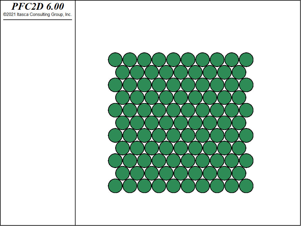
Figure 2: Hexagonal regular packing, low resolution.

To build a polydisperse assembly, a procedure is implemented in a FISH function whose sole argument is the size of the packing. The ball generate gauss option is used, thus ensuring a particle size distribution to follow a Gaussian distribution. A cloud of nonoverlapping balls is generated. The functions are all defined in {“PolydisperseAssembly.p2dat” for 2D; “PolydisperseAssembly.p3dat” for 3D}.

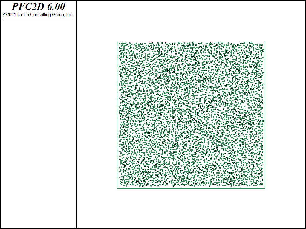
Figure 3: Polydisperse packing, low resolution.

Through the define_meas_parameters function in “MeasureLogic.p2dat”, the measurement parameters are defined. Shown in Fig. 4 and Fig. 5 are screenshots of the measurement regions (nmeas = 5000) as they have been installed to measure the porosity of the cubic regular packing and the polydisperse packing.

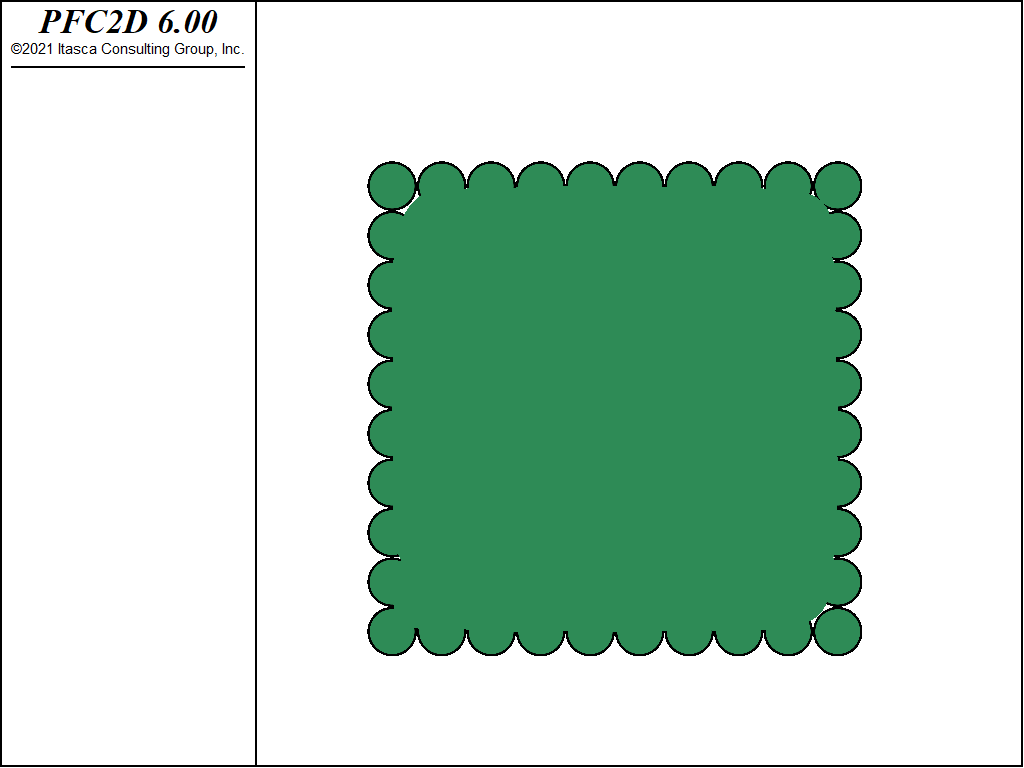
Figure 4: Cubic packing and measurement regions.

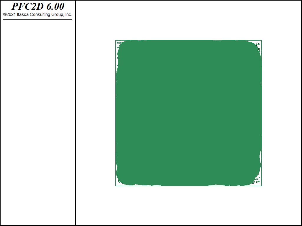
Figure 5: Polydisperse packing and measurement regions.

Results and Discussion

The numerical results are compared to the reference values. The average errors committed using nmeas = 5000 measurement circles and pcntg = 0.0 are reported (Table 2 and Table 3).

In the case of regular assemblies, for the 2D model, we have:

Table 2: Porosity Comparison Regular Assemblies - 2D Model

	Cubic Arrangement		Hexagonal Arrangement
	Low resolution	High Resolution	Low resolution	High Resolution
	9x9	30x30	9x9	30x30
Exact Porosity	0.2146	0.2146	0.0931	0.0931
Average Error [%]	3.87%	0.88%	3.64%	0.74%

Similar results are obtained in the 3D model:

Table 3: Porosity Comparison Regular Assemblies - 3D Model

	Cubic Arrangement		Hexagonal Arrangement
	Low resolution	High Resolution	Low resolution	High Resolution
	9x9	30x30	9x9	30x30
Exact Porosity	0.4764	0.4764	0.2595	0.2595
Average Error [%]	2.24%	0.26%	1.71%	0.20%

The higher the resolution, the lower the average error committed in the porosity measurement. Raw data are stored in four tables (see the table command reference page), one for each examined packing.

Fig. 6 shows the average error, plotted in a logarithmic scale as function of the diameter of the circle employed to measure the porosity, normalized by the average radius of balls. Again, it can be seen that the lowest errors (< 1%, negative values on the logarithmic axis) correspond to the highest resolutions and to the largest measurement regions.

We can make the following observations:

• the measure of the porosity is locally always correct, even more so considering that a tolerance equal to 0 is employed;
• the accuracy of the local measure compared to the global porosity, computed analytically, depends on the representativeness of the area intercepted by the measurement region with respect to the global area, in terms of proportion void/solid;
• it is then clear how a larger measurement region has more chances to provide an accurate measure; and
• it is even clearer how a higher resolution ensures the measurement regions to be more representative of the overall structure.

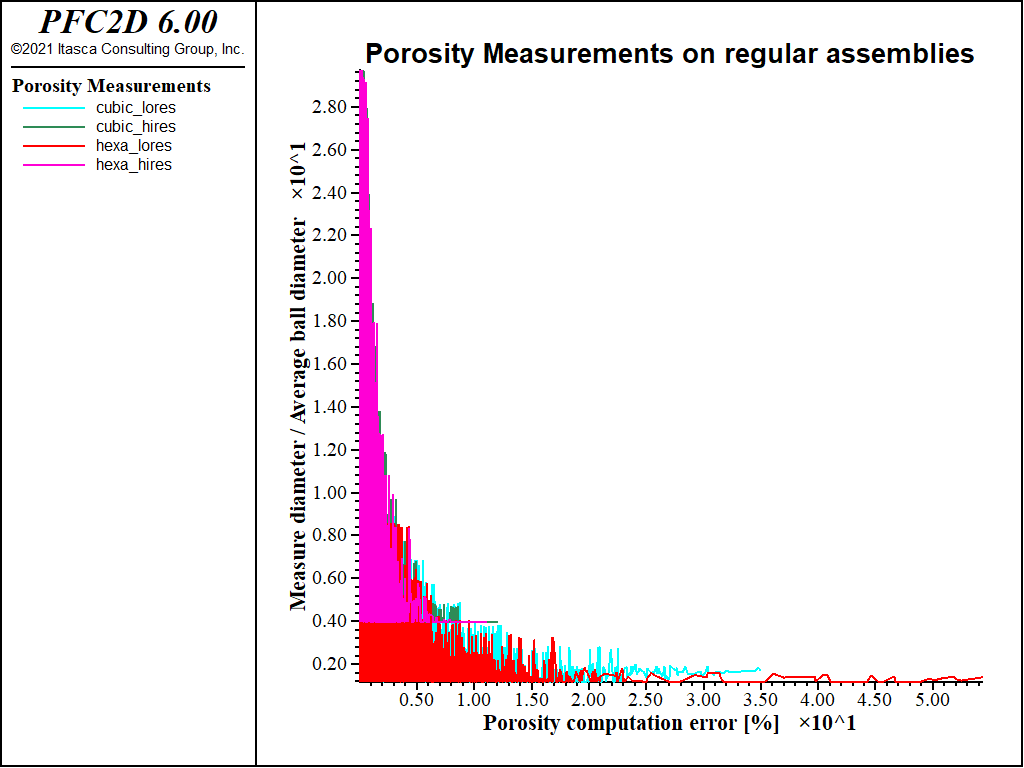
Figure 6: Porosity measurement, regular assemblies - average error [% - log] vs. circle diameter.

We do the same comparison in the case of the polydisperse assembly. The error is plotted in Fig. 7.

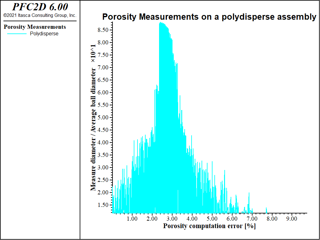
Figure 7: Porosity measurement, polydisperse assembly - average error [% - log] vs. ircle diameter.

The relatively higher errors, with respect to the regular samples, are due to a nonhomogeneous value of porosity throughout the sample. Then, in this case, the employment of larger measurement regions ensures the measures to be less dispersed, even if it seems harder to get rid of a small error (\(\simeq 2\) %).

References

[Deresiewicz1958a]

Deresiewicz, H. “Mechanics of Granular Matter”, in Advances in Applied Mechanics, Vol. 5, pp. 233-306. H. L. Dryden and Th. Von Karman, eds. New York: Academic Press, 1958.

Endnote

[1]

This file may be found in PFC3D under the “verification_problems/MeasurementLogic/MeasurePorosity” folder in the Examples dialog (Help —> Examples on the menu). If this entry does not appear, please copy the application data to a new directory. (Use the menu commands Tools —> Copy App Data …. See the -ref–dlg_copyappdata- section for details. [CS: commented out because UI material not present as of 9/25/17, therefore link is broken. Put back in when UI material is restored])