Rolling Resistance Linear Contact Model: Repose Angle

	Problem Resources
Data Files	Project: Open “ReposeAngle.p2prj” in PFC2D or “ReposeAngle.p3prj” in PFC3D [1]

Introduction

In this example, a granular heap is formed by lifting a container initially filled with balls at rest under gravity. The rolling resistance linear contact model is used, and the simulation is performed several times with varying values of the friction and rolling resistance coefficients to investigate their effect on the final shape of the heap. This example is addressed in PFC2D and PFC3D. Usage of Python scripts to perform batch jobs is demonstrated. In the 3D example, an automated procedure that uses Python scripts to estimate the repose angle of the final heap is proposed.

PFC2D Model

The PFC2D model is described in this section.

Initial State

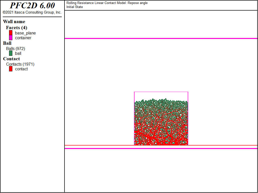
The initial state consists in a granular column (Fig. 1) at rest under gravity in a container. It is built using the data file make_system.p2dat. Selected lines of this file are discussed below.

Figure 1: The initial system.

For convenience, the input parameters are defined as global FISH variables using inline FISH (see here) with the following lines:

; container and balls attributes
[cyl_rad    =  50.0e-3 ] ; container half-width [m]             
[cyl_height =  100.0e-3] ; container height     [m] 
[ravg       =   1.5e-3 ] ; ball average radius  [m] 
[rdev       =   0.5    ] ; ball relative radius deviation [-]
[dens       =   2.0e3  ] ; ball density  [kg/m3]
[poros      =   0.3    ] ; initial porosity [-]

; contact model properties
[emod   = 1.0e6]  ; Young's modulus (deformability method) [Pa]
[kratio = 2.0  ]  ; stiffness ratio (deformability method) [-]
[fric   = 0.01 ]  ; friction coefficient                   [-]
[dpnr   = 0.2  ]  ; normal critical damping ratio          [-]
[dpsr   = 0.2  ]  ; shear critical damping ratio           [-]
[dpm    = 3    ]  ; dashpot mode                           [-]
[rfric  = 0.0  ]  ; rolling resistance coefficient         [-]

The first set of parameters define the container dimensions, as well as the ball size distribution, density, and the porosity of the cloud of balls that is first generated. The container is set to be a 100mm × 100mm square, and the ball radii to have a relative deviation of 0.5 around a mean value of 1.5mm, with a density of 2000.0 kg/m³. The geometry is built as two separate walls: a horizontal base plane that spans the entire domain, and a container made of 3 facets.

; generate the base plane and the container
wall generate id 1               ... 
              name 'base_plane'  ...
              plane

wall create id 100                                                 ...
            name 'container'                                       ...
            vertices [-cyl_rad] 0.0         [-cyl_rad] @cyl_height ...
                     [-cyl_rad] @cyl_height [ cyl_rad] @cyl_height ...
                     [cyl_rad]  @cyl_height [ cyl_rad] 0.0 

The initial cloud of balls is created using the ball distribute command:

ball distribute porosity @poros                      ...
                resolution @ravg                     ...  
                radius [1.0-0.5*rdev] [1.0+0.5*rdev] ...
                box [-1.0*cyl_rad] [1.0*cyl_rad]     ... 
                               0.0 @cyl_height     

The second set of parameters define the contact model properties that will be used in the system. This set of parameters are used to set the default slots of the Contact Model Assignment Table (CMAT), along with the rolling resistance linear contact model:

; set the CMAT default slots
contact cmat default model rrlinear method deformability         ...
                                               emod      @emod   ...
                                               kratio    @kratio ...
                                    property fric      @fric     ...
                                             dp_nratio @dpnr     ...
                                             dp_sratio @dpsr     ...
                                             dp_mode   @dpm      ...
                                             rr_fric   @rfric        

Please refer to the rolling resistance linear contact model section for a detailed description of these properties. Note that at this stage a very low value of the friction coefficient is used, and the rolling resistance coefficient is set to zero. These values are used to produce a relatively dense final state. Also note that the contact Young’s modulus is set to 1MPa (using the contact model’s deformability method). This value is sufficient to ensure that the system remains within the rigid grain limit (i.e. the ratio between the contact Young’s modulus and the maximal stress at the bottom of the column is large enough, or inversely the magnitude of the overlaps are small compared to the contacting ball diameters, so that increasing further the contact stiffness would not affect the results) while optimizing the estimated timestep.

Finally, gravity is set as well as the ball density and local damping coefficient attributes; the system is subsequently solved to equilibrium with the following commands:

; bring to rest under gravity loading                                      
ball attribute density @dens damp 0.7
model cycle 1000 calm 10
model gravity 9.81
model solve
ball attribute damp 0.0
model save 'system_ini.p2sav'

Note the use of the calm keyword with the model cycle command to efficiently remove the energy arising from the large initial overlaps inherent to the use of the ball distribute command. Local damping is set to a large value of 0.7 during this phase, as we are only interested in the final equilibrated state (and not in the path followed by the system). It is reset to zero before proceeding to the heap formation.

Heap Formation

The final heap configuration is formed by lifting the container wall upwards. This is done using the following set of commands (in the file move_container.p2dat):

[cyl_vel = 5.0e-2]  ; upwards velocity [m/s] 
model mechanical time-total 0.0
contact cmat default property fric @fric rr_fric @rfric
contact property fric @fric rr_fric @rfric
wall attribute velocity-y @cyl_vel range id 100 by wall
ball attribute displacement multiply 0.0
model solve time [0.75*cyl_height/cyl_vel]
wall attribute velocity-y 0.0 range id 100 by wall
model solve ratio-average 1e-5
model save [string.build('system_final-fric%1-rfric%2.p2sav',fric,rfric)]

Note that the default slots of the CMAT are changed prior to cycling. This ensures that new contacts that will be formed will use updated values of the friction and rolling resistance coefficients. In addition, the values of these properties are also altered at existing contacts.

This file is not intended to be executed directly. Instead, it can be sequentially invoked from another datafile, in order to perform a series of simulations with different parameter sets. For instance, the file do_analysis.p2dat will perform 3 simulations with a friction coefficient of 0.5, and a rolling resistance coefficient of 0.1, 0.5 and 1.0:

model restore 'system_ini'
[fric  = 0.5]
[rfric = 0.1]
program call 'move_container.p2dat'
;
model restore 'system_ini'
[fric  = 0.5]
[rfric = 0.5]
program call 'move_container.p2dat'
;
model restore 'system_ini'
[fric  = 0.5]
[rfric = 1.0]
program call 'move_container.p2dat'

Alternatively, Python scripts may be used to perform batch jobs, as demonstrated by the file do_analysis.py:

import itasca

fric  = [0.25,0.5]
rfric = [0.05,0.1,0.25,0.5,0.6]

for f in fric:
  for rf in rfric:
    itasca.command("""
                     model restore 'system_ini'
                     [fric  = {0}]
                     [rfric = {1}]
                     program call 'move_container.p2dat'
                   """.format(f,rf)
    )

Contrary to FISH, the Python state is independent from the PFC model state. In this specific case, this provides the ability to invoke restore commands inside of a Python loop. This specific example defines two lists of values, and uses nested loops to explore this parameter space.

The final states for all values of the rolling friction coefficient are shown in Fig. 2 for \(\mu=0.25\) and Fig. 3 for \(\mu=0.5\).

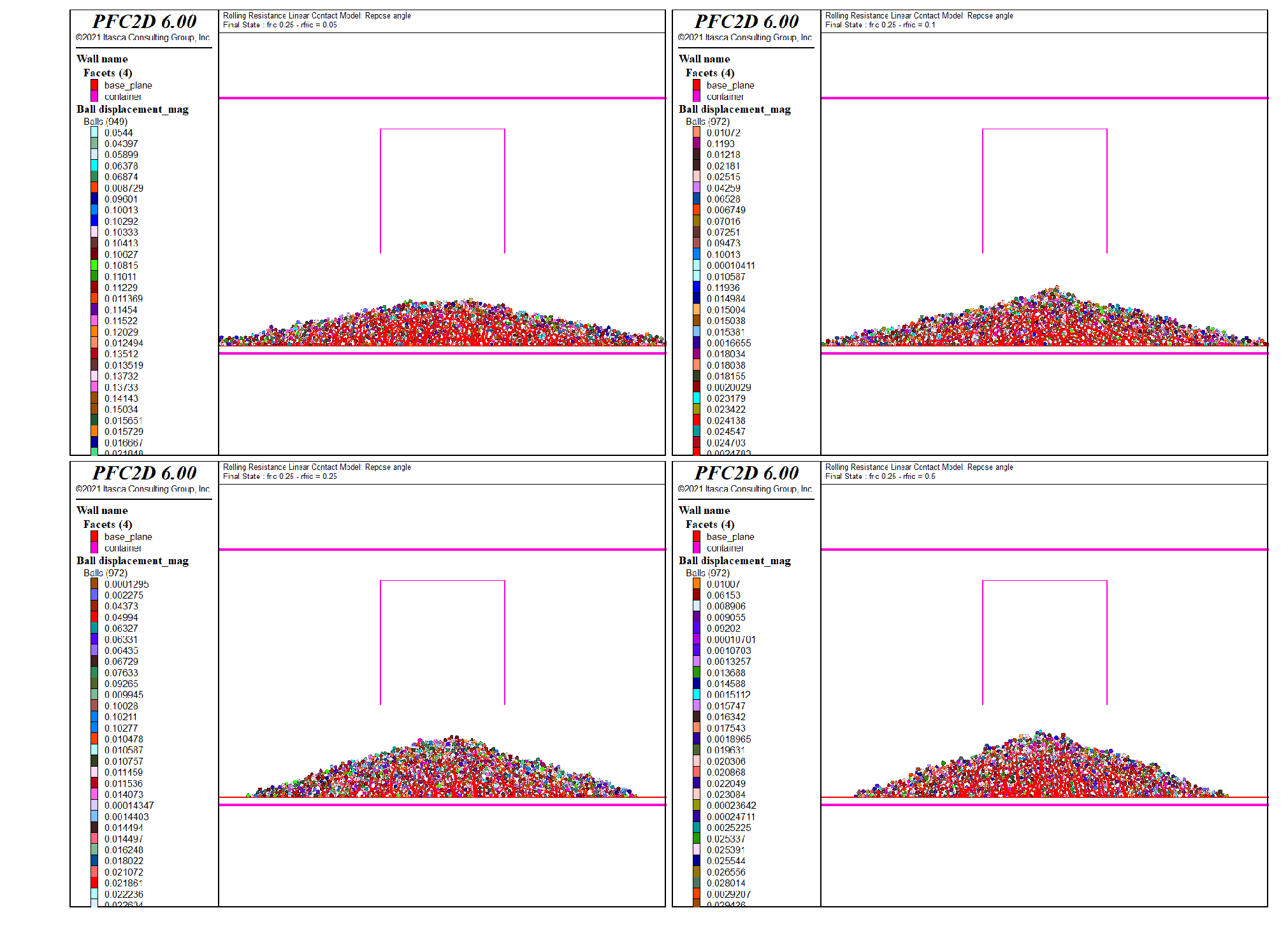
Figure 2: The final systems with \(\mu = 0.25\) and \(\mu_r = 0.05\) (top left), \(\mu_r = 0.1\) (top right), \(\mu_r = 0.25\) (bottom left) and \(\mu_r = 0.5\) (bottom right).

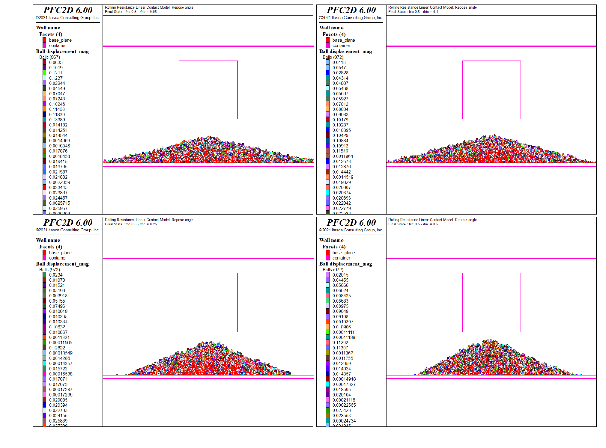
Figure 3: The final systems with \(\mu = 0.5\) and \(\mu_r = 0.05\) (top left), \(\mu_r = 0.1\) (top right), \(\mu_r = 0.25\) (bottom left) and \(\mu_r = 0.5\) (bottom right).

The influence of the friction and rolling friction coefficients can be qualitatively discussed from these two figures. At a constant coefficient of friction, the repose angle of the heap increases with increasing value of the rolling friction coefficient. However this increase seems to plateau if the rolling friction coefficient is equal or greater than the friction coefficient (see for instance the bottom figures in Fig. 2). Similarly, at constant rolling friction coefficient, the angle of repose also increases with increasing friction coefficient.

The present model lacks a systematic procedure to estimate the repose angle of the final heap, which would allow a quantitative comparison of the results. This issue is addressed in the PFC3D model described below.

PFC3D Model

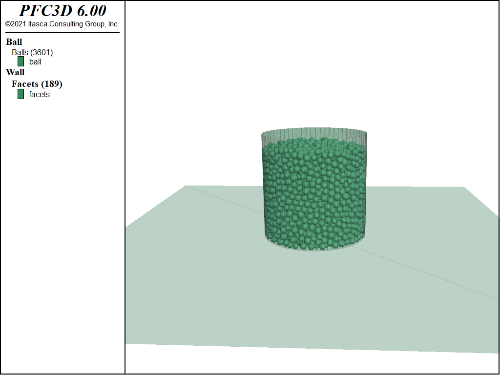
The PFC3D model is similar to the PFC2D model described above, with the difference that the container is a cylinder, and that the balls have an average radius of 3.0 mm with a relative deviation of 0.25 to limit the size of the model. The initial system (Fig. 4) is constructed using the file make_system.p3dat, and the heap formation is simulated using the file do_analysis.py, which sequentially calls move_container.p2dat to perform multiple runs with different values of the friction and rolling friction coefficients.

The 3D example also uses an automated procedure to estimate the repose angle of the 3D heap. This procedure uses the Python scripts discussed below.

Figure 4: The initial system.

Post-treatment: Measure of the Angle of Repose

Post-processing of the final states is performed using the Python script post_treat.py, replicated below:

import utils
import matplotlib.pyplot as plt
fric  = [0.2,0.6]
rfric = [0.1,0.2,0.4,0.6,0.8]

val = []
conf = []
leg = []
for f in fric:
  ra = []
  ci = []
  for rf in rfric:
    p,c = utils.fit_cone('system_final-fric{0}-rfric{1}.p3sav'.format(f,rf))
    ra += [p]
    ci += [c]  
  val += [ra]
  conf += [ci] 
  leg += [r'$\mu={0}$'.format(f)]
  
plt.close('all')
for i, v in enumerate(val):
  plt.errorbar(rfric , val[i],yerr=ci[i])
plt.legend(leg,loc=2)
plt.title("Repose Angle vs Rolling Friction Coefficient")
plt.xlabel("Rolling Friction Coef. [-]")
plt.ylabel("Angle of Repose [$^{\circ}$]")
plt.axis([0, 0.9, 0, 40])
plt.grid(True)
plt.draw()

For each pair of (friction,rolling friction) coefficients, the code in this file invokes the function fit_cone, which is defined in the utility file utils.py. The purpose of this function is to identify balls on the free surface of the heap, and to fit a cone surface based on the location of those balls. It uses algorithms available in the SciPy Python module : a KD-Tree for quick identification of the balls on the free-surface of the heap (using a neighboring distance equal to the average diameter of the balls), and a curve-fitting function to fit a cone on the location of the identified balls (note that balls within one maximal diameter from the base plane or from the apex of the heap are ignored).

Fig. 5 shows the finals state for \(\mu = 0.6\) and \(\mu_r = 0.8\) (top and bottom left), and \(\mu = 0.2\) and \(\mu_r = 0.1\) (top and bottom right). The balls identified on the free surface are shown in a different color, and the fitted cone is shown in the bottom plots. This figure shows that the proposed procedure seems reasonably accurate in estimating the repose angle of the heap for the extreme sets of parameters.

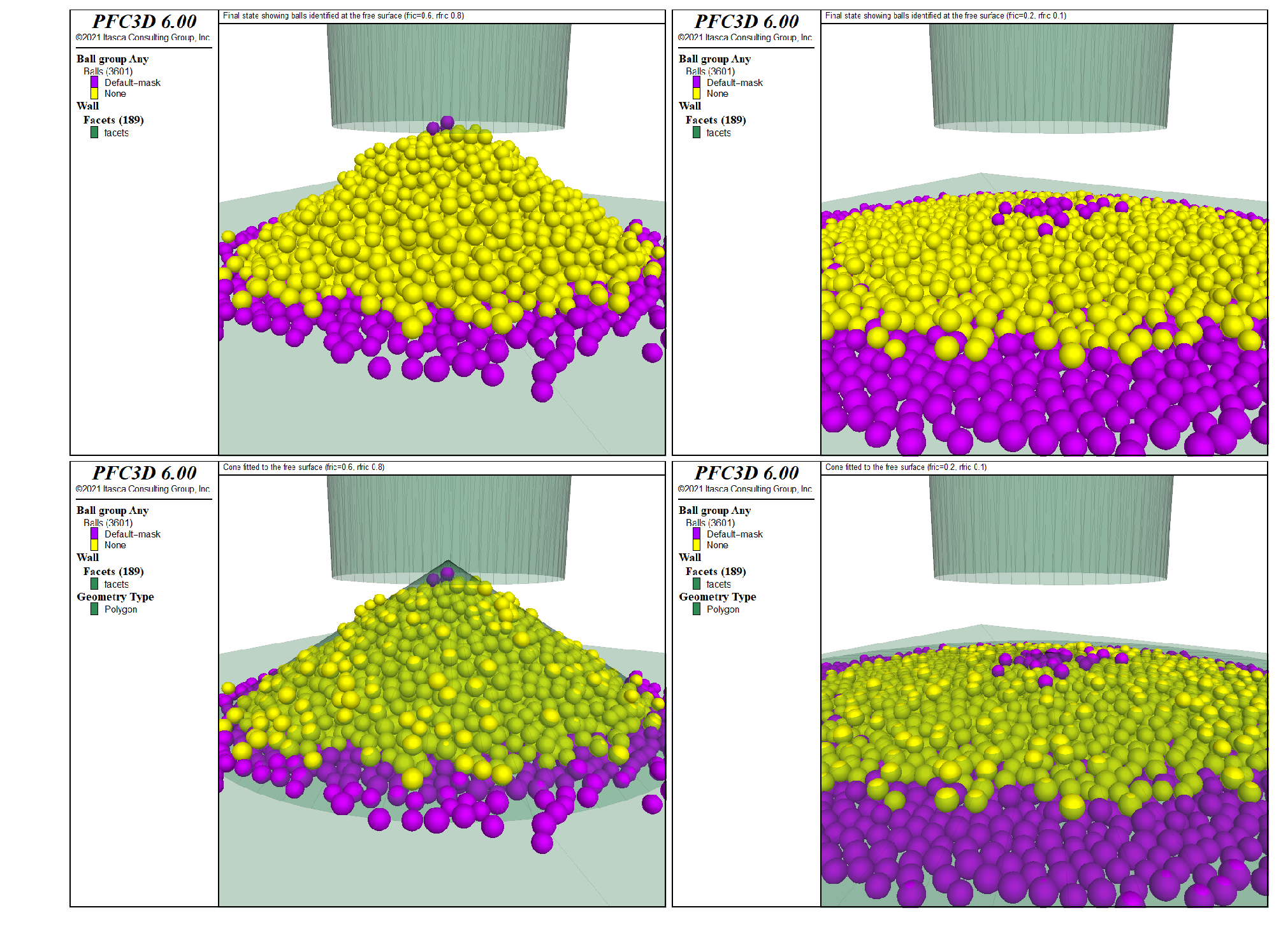
Figure 5: Final state showing the balls identified at the free surface and the fitted cone for \(\mu = 0.6\) and \(\mu_r = 0.8\) (top and bottom left), and \(\mu = 0.2\) and \(\mu_r = 0.1\) (top and bottom right).

Results

Fig. 6 shows the evolution of the estimated repose angle with increasing rolling friction coefficient, for \(\mu = 0.2\) and \(\mu = 0.6\). The error bars indicate, for each estimation, the 95% student-t based confidence interval of the estimated value. The results confirm and quantify the trends observed in the 2D model: the repose angle increases with increasing friction and rolling friction coefficients, and for a constant friction coefficient, reaches a plateau when the rolling friction coefficient becomes larger than a value that is close to that of the friction coefficient. The test should be repeated with different sets of parameters and with different initial geometries of the packing (i.e. different random seed numbers) to obtain better statistics, and an iso-value map of the estimated repose angle could be produced, as done in [Wensrich2012] for a model similar to the one presented here. Also, other parameters, such as the size of the system, the particle size-distribution, or the properties of the contacts with the base plane will affect the results and this example could easily be augmented to assess their influence.

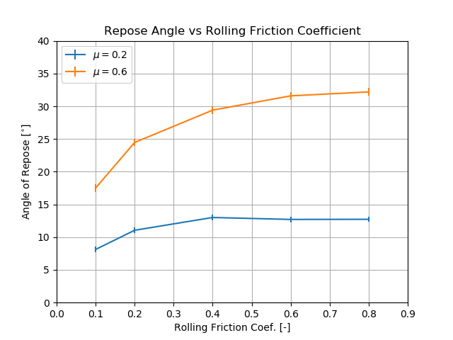
Figure 6: Estimated repose angle versus rolling friction coefficient, for \(\mu = 0.2\) and \(\mu = 0.6\).

Discussion

This example exercises the rolling resistance linear contact model in the situation of a heap formed by moving upwards a container initially filled with balls at rest under the action of gravity, both with PFC2D and PFC3D. Usage of Python scripts to perform sensitivity analyses and post-process the results is demonstrated. The evolution of the repose angle of the heap with increasing friction and rolling friction coefficients is investigated, and conforms to the expected behavior and to results from the literature A more exhaustive analysis, including the investigation of the size of the system, particle size-distribution, and the properties of the contacts with the base plane should be conducted for a more detailed discussion.

Endnote

[1]

These files may be found in PFC2D or PFC3D under the “verification_problems/rolling_resistance/repose_angle” folder in the Examples dialog (Help —> Examples on the menu). If this entry does not appear, please copy the application data to a new directory. (Use the menu commands Tools —> Copy App Data …. See the “Copy Application Data” section for details.)