Transient Thermal Response of Sheet with Constant Temperature Boundaries

	Verification Resources
Data Files	Project: open “TransientSheet.p2prj,”[1] in PFC2D

A planar sheet of width \(L\) is initially at a uniform temperature of 0°C. The left side of the sheet is exposed to a constant temperature of 100°C, while the right side is kept at 0°C. The sheet eventually reaches an equilibrium state at a constant heat flux and unchanging temperature distribution. The analytical solution for temperature within the sheet as a function of distance from the left side, \(x\), and time, \(t\), is given by [Crank1975]

(1)\[\frac{T(x,t)}{T_1} = 1 - \frac{x}{L} - \frac{2}{\pi} \sum_{n=1}^{\infty} e^{- \kappa n^2 \pi^2 t / L^2} \left(\frac{\sin (n \pi x / L)}{n}\right)\]

where \(T_1\) is the temperature at the left side of the sheet (equal to 100°C), and \(\kappa\) is the thermal diffusivity given by

(2)\[\kappa = \frac{k}{\rho_t C_v}\]

where \(k\) is the thermal conductivity, \(\rho_t\) is the material density, and \(C_v\) is the specific heat at constant volume.

Numerical Model

This thermal problem is one-dimensional and can be modeled as a thin slice of material with constant temperatures applied to its left and right boundaries and adiabatic conditions on the upper and lower boundaries to represent thermal symmetry planes.

For this example, we create two different PFC2D models consisting of a cubic packing and a hexagonal packing (see Figures 1 and 2). For these two uniform packings, the porosity and the thermal resistance can be expressed analytically. The porosity is given by [Deresiewicz1958b]:

(3)\[\begin{split}n = \begin{cases} 1 - \pi / 4 & \mbox{ , (cubic pack)} \\ 1 - \pi / 2 \sqrt{3} &\mbox{ , (hexagonal pack)} \end{cases}\end{split}\]

The thermal resistance is found by applying Equation (28) of the PFC Thermal Formulation section to a control volume that surrounds one particle, and noting that the length of each thermal pipe contained within the control volume equals the particle radius, \(R\), to yield

(4)\[\begin{split}\eta = \frac{1}{kRt} \begin{cases} \frac{1}{2} & \mbox{ , (cubic pack)} \\ \frac{3}{2 \sqrt{3}} & \mbox{ , (hexagonal pack)} \end{cases}\end{split}\]

where \(t\) is the disk thickness (equal to unity in this case). The data file used to perform the simulation is “transient_sheet.p2dat”. It makes use of FISH functions defined in “transient_sheet-utils.p2fis”. Thermal properties and boundary conditions are specified, and then each model is run for 50 and 200 cycles, until the thermal equilibrium state is reached (using the model solve command). The normalized temperature distributions at the increasing thermal times for the cubic- and hexagonal-packed specimens are plotted along with the analytical solutions in Figures 3 and 4. There is a good match between the PFC2D responses and the analytical solutions.

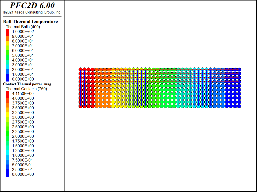
Figure 1: Contour of ball temperature and thermal power vector field (PFC2D cubic pack).

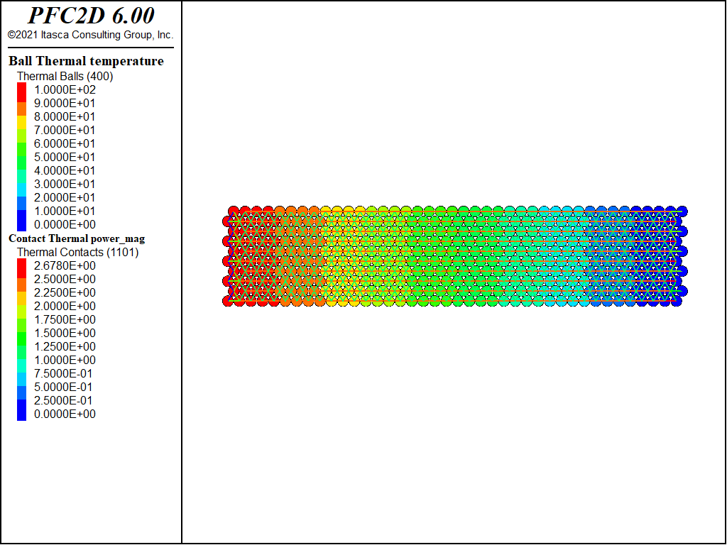
Figure 2: Contour of ball temperature and thermal power vector field (hexagonal pack).

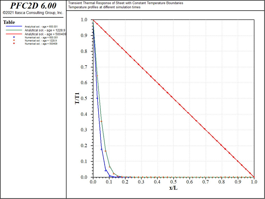
Figure 3: Modeled and analytical normalized temperature distributions for increasing thermal time (cubic pack).

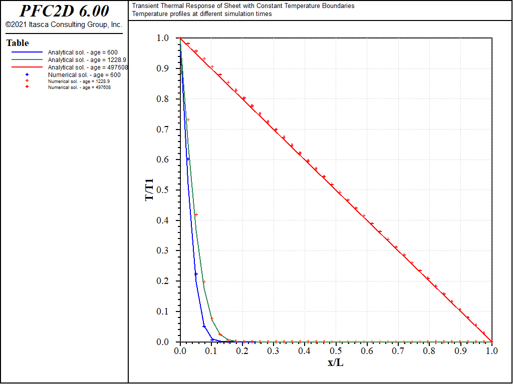
Figure 4: Modeled and analytical normalized temperature distributions for increasing thermal time (hexagonal pack).

References

[Crank1975]

Crank, J. The Mathematics of Diffusion, 2nd Ed. Oxford: Oxford University Press, 1975.

[Deresiewicz1958b]

Deresiewicz, H. “Mechanics of Granular Matter,” in Advances in Applied Mechanics, Vol. 5, pp. 233-306. H. L. Dryden and Th. von Karman, eds. New York: Academic Press, 1958.

Endnote

[1]

This file may be found in PFC2D under the “verfication_problems/transient_sheet” folder in the Examples dialog (Help —> Examples on the menu). If this entry does not appear, please copy the application data to a new directory. (Use the menu commands Tools —> Copy App Data …. See the Copy Application Data section for details.)