Heated Specimen with Fixed Boundaries

	Verification Resources
Data Files	Project: open “ConstrainedExpansion.p3prj,”[1] in PFC3D

A temperature increment, \(\Delta T\), is applied to a cubic specimen with constrained boundaries. The surrounding six walls are fixed to constrain the expansion of the specimen, and thermally induced stresses are measured and compared with the analytical values.

Analytical Values

The stress-strain relation with thermally induced strain is given by Equation (1) ([Timoshenko1970a]):

(1)\[\begin{split}\epsilon_x &= {1 \over E} {\big[ \sigma_x - \nu (\sigma_y+\sigma_z) \big]} + \alpha_t \Delta T \\ \epsilon_y &= {1 \over E} {\big[ \sigma_y - \nu (\sigma_z+\sigma_x) \big]} + \alpha_t \Delta T \\ \epsilon_z &= {1 \over E} {\big[ \sigma_z - \nu (\sigma_x+\sigma_y) \big]} + \alpha_t \Delta T\end{split}\]

where \(E\) and \(\nu\) are the Young’s modulus and the Poisson’s ratio, respectively. Also, \(\alpha_t\) is the coefficient of linear thermal expansion.

The analytical values for thermally induced stresses on the isotropic specimen are given by Equation (2), substituting \(\sigma_x=\sigma_y=\sigma_z\) and \(\epsilon_x=\epsilon_y=\epsilon_z=0\) into Equation (1):

(2)\[\sigma_x = \sigma_y = \sigma_z = -\alpha_t \Delta T {E \over {1-2\nu}}\]

Model and Results

The file “constrained_expansion.p3dat” is used for this example. A 2 × 2 × 2 m specimen is created. It comprises approximately 4000 balls with uniform size distribution (radius range from 0.05 to 0.08 m) and a porosity of 0.38. Once the specimen is generated and equilibrated under an isotropic stress state of 100kPa, contact bonds are installed at ball-ball contacts.

The stress and strains are measured using a measurement sphere with a radius of 0.95 m centered within the specimen, and the stresses are also measured on the boundary walls. In PFC, the particle thermal-expansion coefficient is the same as the coefficient of linear thermal expansion: \(\alpha_t\) = 3 × 10^-6/°C in this case.

The increment of stress measured at the boundary walls during thermal isotropic constrained expansion are:

(3)\[\begin{split}\Delta \sigma_xx &= -2.98 \times 10^5 \\ \Delta \sigma_yy &= -2.95 \times 10^5 \\ \Delta \sigma_zz &= -3.04 \times 10^5\end{split}\]

Figures 1 and 2 shows the contact forces colored by magnitude before and after thermal expansion.

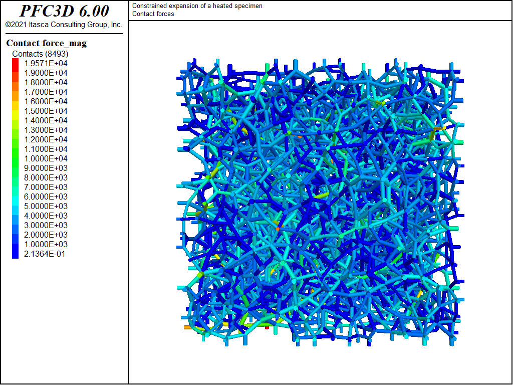
Figure 1: Contact forces before thermal isotropic constrained expansion.

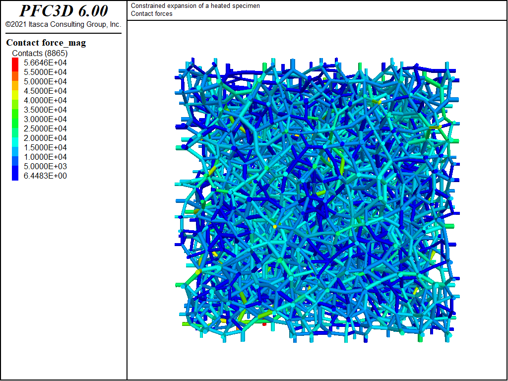
Figure 2: Contact forces after thermal isotropic constrained expansion.

To evaluate the analytical solution, the Young’s modulus, \(E\), and the Poisson’s ratio, \(\nu\), are computed by a confined compression test of the specimen at a lateral confinement 100 kPa.

(4)\[\begin{split}E &= 366 \ {\rm MPa} \\ \\ \nu &= 0.314\end{split}\]

Incorporating these values into Equation (2) leads to:

(5)\[\sigma_x = \sigma_y = - 2.95 \times 10^5\]

This value compares well with the measured stress increments reported in (3). The difference may be attributed to the fact that the specimen is not completely uniform; the arbitrary packing produces heterogeneity in the material microstructure.

Reference

[Timoshenko1970a]

Timoshenko, S. P., and J. N. Goodier. Theory of Elasticity, 3rd Ed. New York: McGraw-Hill, 1970.

Endnote

[1]

This file may be found in PFC3D under the “verfication_problems/constrained_expansion” folder in the Examples dialog (Help —> Examples on the menu). If this entry does not appear, please copy the application data to a new directory. (Use the menu commands Tools —> Copy App Data …. See the Copy Application Data section for details.)