Heated Specimen with Free Boundaries

	Verification Resources
Data Files	Project: open “FreeExpansion.p3prj,”[1] in PFC3D

A temperature change, \(\Delta T\), is applied to a cubic specimen with unconstrained boundaries. The thermally induced strains are measured and compared with analytical values for an isotropic elastic continuum.

Analytical Values

The stress-strain relation with thermally induced strain is given by Equation (1) ([Timoshenko1970b]):

(1)\[\begin{split}\epsilon_x &= {1 \over E} {\big[ \sigma_x - \nu (\sigma_y+\sigma_z) \big]} + \alpha_t \Delta T \\ \epsilon_y &= {1 \over E} {\big[ \sigma_y - \nu (\sigma_z+\sigma_x) \big]} + \alpha_t \Delta T \\ \epsilon_z &= {1 \over E} {\big[ \sigma_z - \nu (\sigma_x+\sigma_y) \big]} + \alpha_t \Delta T\end{split}\]

where \(E\) and \(\nu\) are the Young’s modulus and the Poisson’s ratio, respectively. Also, \(\alpha_t\) is the coefficient of linear thermal expansion.

The analytical values for the thermally induced strains with free boundaries are given by Equation (2):

(2)\[\epsilon_x = \epsilon_y = \epsilon_z = \alpha_t \Delta T\]

Model and Results

The file “free_expansion.p3dat” is used for this example. A 2 × 2 × 2 m specimen is created. It comprises approximately 4000 balls with uniform size distribution (radius range from 0.05 to 0.08 m), with a porosity of 0.36. Once the specimen is generated, contact bonds are installed at ball-ball contacts, the surrounding walls are deleted, and the specimen is brought to equilibrium.

The strains are measured using a measurement sphere with a radius of 0.95 m, centered within the specimen. In PFC, the particle thermal-expansion coefficient is the same as the coefficient of linear thermal expansion: \(\alpha_t\) = 3 × 10^-6/°C, in this case.

The expected strains for \(\Delta T\) = +100°C are

(3)\[\epsilon_x = \epsilon_y = \epsilon_z = 3.0 \times 10^{-4}\]

The expected strains for \(\Delta T\) = -100°C are

(4)\[\epsilon_x = \epsilon_y = \epsilon_z = -3.0 \times 10^{-4}\]

Figure 1 and Figure 2 show displacement vectors resulting from the positive and negative temperature change; they show an isotropic expansion and isotropic contraction, respectively. Figure 3 and Figure 4 show histories of strain recorded during the expansion and contraction phases respectively.

The result of the simulation is in accordance with the analytical solution.

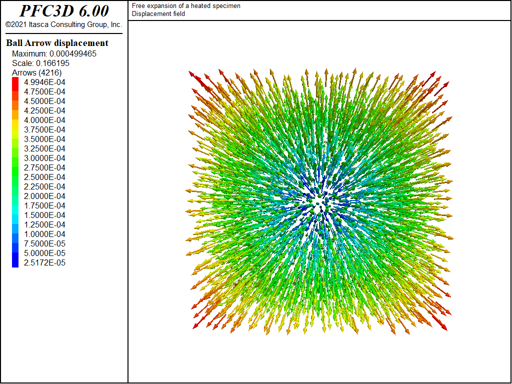
Figure 1: Displacement field at the end of thermal isotropic expansion.

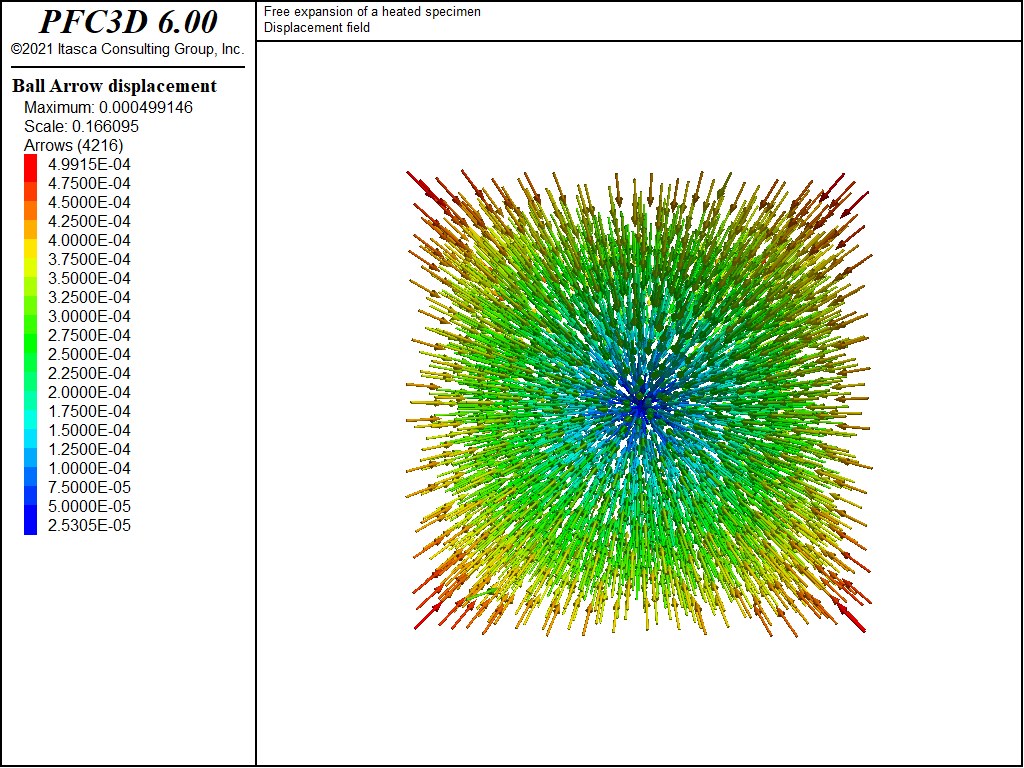
Figure 2: Displacement field at the end of thermal isotropic contraction.

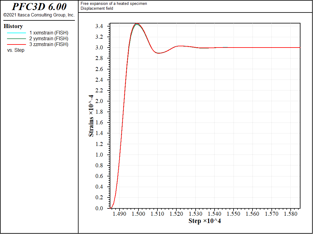
Figure 3: Strain histories at the end of thermal isotropic expansion.

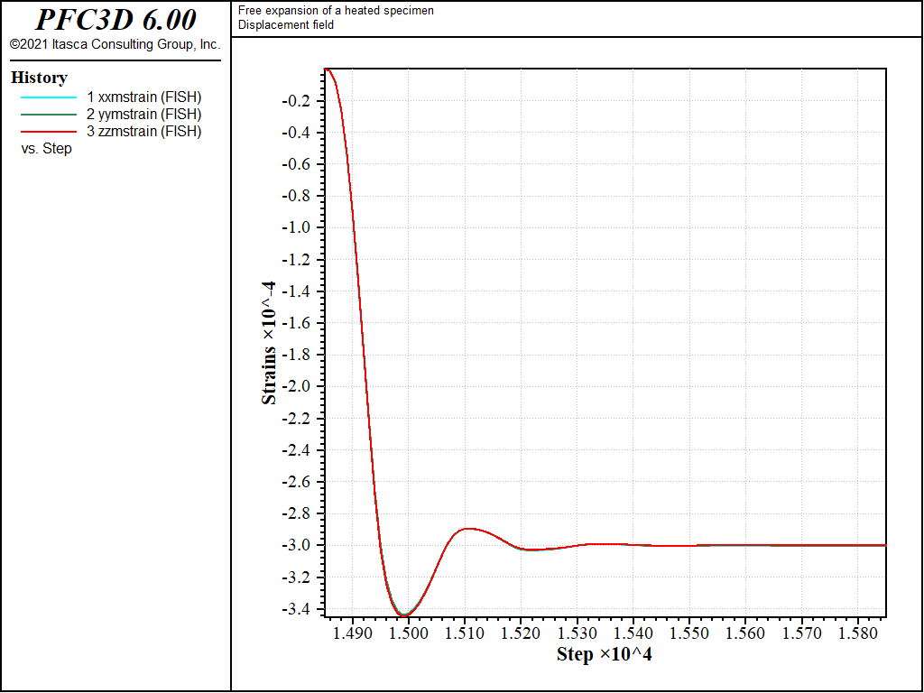
Figure 4: Strain histories at the end of thermal isotropic contraction.

References

[Timoshenko1970b]

Timoshenko, S. P., and J. N. Goodier. Theory of Elasticity, 3rd Ed. New York: McGraw-Hill, 1970.

Endnote

[1]

This file may be found in PFC3D under the “verfication_problems/constrained_expansion” folder in the Examples dialog (Help —> Examples on the menu). If this entry does not appear, please copy the application data to a new directory. (Use the menu commands Tools —> Copy App Data …. See the Copy Application Data section for details.)