
Numerical Thermal Formulation
Introduction
The thermal option of 3DEC allows simulation of transient heat conduction in materials, and development of thermally induced displacements and stresses. This option has the following specific features:
- Any of the mechanical models may be used with the thermal model.
- Temperature, flux, convective and adiabatic boundary conditions may be prescribed.
- Heat sources may be inserted into the material as either point sources or volume sources. These sources may decay exponentially with time.
- Both explicit- and implicit-solution algorithms are available.
- The thermal option provides for one-way coupling to the mechanical stress calculations through the thermal expansion coefficients.
- Temperatures can be accessed via FISH.
- Coupling between fluid flow in fractures and the thermal logic is available.
The thermal option also allows modeling of transient thermal convection in fractures filled with a moving fluid. In this version of the code, fluid thermal expansion is not considered in the fluid thermo-mechanical coupling.
This section contains descriptions of the thermal formulation and the 3DEC input commands for thermal analysis. Thermal conduction is considered in the Heat Conduction section; thermal convection is reviewed in the Heat Convection section. Recommendations for solving thermal problems are also provided, along with several verification problems. Refer to these examples as a guide to creating 3DEC models for thermal analysis and coupled thermal-stress or thermal-fluid flow analysis.
Heat Conduction
Introduction
The logic for heat conduction through a solid is available for deformable blocks. (It is not activated for rigid blocks.) By default, convection is off and heat is conducted across the blocks using an interpolation procedure. (The fractures are not seen by the flow of heat in this case.) Fluid-thermal coupling can also be activated. (This topic is addressed in the Heat Convection section.)
Mathematical Model Description
The variables involved in heat conduction in 3DEC are temperature and the three components of the heat flux. These variables are related through the energy-balance equation and transport laws derived from Fourier’s law of heat conduction. Substitution of Fourier’s law into the energy-balance equation yields the differential equation of heat conduction, which may be solved for particular geometries and properties, given specific boundary and initial conditions. Thermal volumetric-strains are introduced into the incremental mechanical constitutive laws to account for thermomechanical coupling.
Conventions and Definitions
As a notation convention, the symbol \(a_i\) denotes component \(i\) of the vector [ \(a\) ] in a Cartesian system of reference axes; \(A_{ij}\) is component (\(i, j\)) of tensor [ \(A\) ]. Also, \(f_{,i}\) is used to represent the partial derivative of \(f\) with respect to \(x_i\). (\(f\) can be a scalar variable or a vector component.)
The Einstein summation convention applies only to indices \(i\), \(j\), and \(k\), which take the values 1, 2, 3 for components that involve spatial dimensions. The indices may take any values when used in matrix equations.
SI units are used to illustrate parameters and dimensions of variables. See Systems of Units for Thermal Analysis for conversions to other systems of units.
The following dimensionless numbers are useful in the characterization of transient heat conduction.
Characteristic length:
Thermal diffusivity:
where:
\(k\) is the thermal conductivity;
\(\rho\) is the density; and
\(C_v\) is the specific heat at constant volume.
Characteristic time:
Energy-Balance Equation
The differential expression of the energy balance has the form
where \(q_i\) is the heat-flux vector in [\(W/m\)2], \(q_v\) is the volumetric heat-source intensity in [\(W/m\)3], and \(\zeta\) is the heat stored per unit volume in [\(J/m\)3]. In general, temperature changes may be caused by changes in both energy storage and volumetric strain, \(\epsilon\). And the thermal constitutive law relating those parameters may be expressed as
where \(M_{th}\) and \(\beta_{th}\) are material constants, and \(T\) is temperature.
In 3DEC, we consider a particular case of this law for which \(\beta_{th}\) = 0 and \(M_{th}\) = \(1 \over {\rho C_v}\). \(\rho\) is the mass density of the medium in [\(kg/m\)3], and \(C_v\) is the specific heat at constant volume in [\(J/kg\) °\(C\)]. The hypothesis here is that strain changes play a negligible role in influencing the temperature — a valid assumption for quasi-static mechanical problems involving solids and liquids. Accordingly, we may write
Substitution of Equation (6) in Equation (4) yields the energy-balance equation
Note that for nearly all solids and liquids, the specific heats at constant pressure and at constant volume are essentially equal. Consequently, \(C_v\) and \(C_p\) can be used interchangeably.
Transport Law
The basic law that defines the relation between the heat-flux vector and the temperature gradient is Fourier’s law. For a stationary, homogeneous, isotropic solid, this constitutive law is given in the form
where \(T\) is the temperature [°C] and \(k\) is the thermal conductivity in [\(W/m °C\)].
Boundary and Initial Conditions
Substitution of Equation (8) for \(q_i\) in Equation (7) yields the differential equation for heat conduction. Initial conditions correspond to a given temperature field. Boundary conditions are generally expressed in terms of temperature or the component of the heat-flux vector normal to the boundary. In this version of 3DEC, four types of conditions are considered. These correspond to: (1) given temperature; (2) given component of the flux normal to the boundary; (3) convective boundaries; and (4) insulated (adiabatic) boundaries.
In 3DEC, a convective boundary condition has the form
where \(q_n\) is the component of the flux normal to the boundary in the direction of the exterior normal, \(h\) is the convective heat-transfer coefficient [\(W/m\)2 °\(C\)], \(T\) is the temperature of the boundary surface and \(T_e\) is the temperature of the surrounding fluid [°C]. Note that in the numerical formulation used in 3DEC, boundaries are adiabatic by default.
Mechanical Coupling – Thermal Strains
Solving thermal-stress problems requires reformulation of the incremental stress-strain relations, which is accomplished by subtracting from the total strain increment that portion due to temperature change. Because free thermal expansion results in no angular distortion in an isotropic material, the shearing-strain increments are unaffected. The thermal-strain increments associated with the free expansion corresponding to temperature increment \(\Delta T\) have the form
where \(\alpha t\) [1/ °\(C\)] is the coefficient of linear thermal expansion, and \(\delta_{ij}\) is the Kronecker delta.
The differential equation of motion and the rate of strain-velocity relations are based upon mechanical considerations, and are unchanged for thermomechanics.
Numerical Formulation
The energy-balance equation (Equation (7)) and Fourier’s law (Equation (8)) are solved in 3DEC using a finite-difference approach based on a medium discretization into zones (tetrahedra). The numerical scheme rests on a nodal formulation of the energy-balance equation. This formulation is equivalent to the mechanical formulation (presented in the 3DEC Theory and Background section) that leads to the nodal form of Newton’s law. It is obtained by substituting the temperature, heat-flux vector, and temperature gradient for velocity vectors, stress tensors, and strain-rate tensors, respectively. The resulting system of ordinary differential equations is solved using two modes of discretization in time, corresponding to explicit and implicit formulations. The principal results are summarized below.
Finite-Difference Approximation to Space Derivatives
By convention, the nodes of a tetrahedron are referred to locally by a number from 1 to 4, face \(n\) is opposite node \(n\), and the superscript (\(f\)) relates to the value of the associated variable on face \(f\).
A linear temperature variation is assumed within a tetrahedron; the temperature gradient, expressed in terms of nodal values of the temperature by application of the Gauss divergence theorem, may be written as
where [\(n\)]\(^(l)\) is the exterior unit vector normal to face \(l\), \(S\) is the face surface area and \(V\) is the tetrahedron volume.
Nodal Formulation of the Energy-Balance Equation
The energy-balance Equation (8) may be expressed as
where
is the equivalent of the instantaneous “body forces” used in the mechanical node formulation. First consider a single tetrahedron. Using this analogy, the nodal heat \(Q_e^n [W]\), \(n\) = 1,4, in equilibrium with the tetrahedron heat flux and body forces, may be expressed as
where
and
In principle, the nodal form of the energy-balance equation is established by requiring that, at each global node, the sum of equivalent nodal heat (\(-Q_e^n\)) from all tetrahedra meeting at the node and nodal contribution (\(Q_w^n\)) of applied boundary fluxes and sources be zero.
The components of the tetrahedron heat-flux vector in Equation (15) are related to the temperature gradient by means of the transport law (see Equation (8)). In turn, the components of the temperature gradient can be expressed in terms of the tetrahedron’s nodal temperatures, using Equation (11).
In order to save computer time, a zone formulation is adopted in 3DEC. At each node, \(n\), of a particular zone, the sum, \(Q_z^n\), of contributions from all tetrahedra belonging to the zone and meeting at the node is formed and divided by two for two overlays. Local zone matrices, [\(M\)], that relate nodal zone values, \(Q_z^n\), to nodal zone temperatures, \(T^n\) (\(n\) = 1,4), are assembled. These matrices being symmetrical, 10 components are computed and saved at the beginning of the computation and updated every 10 steps in large-strain mode. By definition of zone matrices, we have
where [\(T\)] is the local vector of nodal zone temperatures.
In turn, global nodal values, \(Q_T^n\), are obtained by superposition of zone contributions. Taking some liberty with the notation, we write for each global node \(n\),
where [\(C\)] is the global matrix, and [\(T\)] is, in this context, the global vector of nodal temperatures.
Returning to our previous consideration, we write
where, for simplicity of notation, the \(\sum\) sign is used to represent summation of the contributions at global node \(n\) of all zones meeting at that node. Using Equation (14) in Equation (19), we obtain, after some manipulations,
where \(Q_T^n\) is a function of the nodal temperatures defined in Equation (18), and \(\sum Q_{app}^n\) is the known contribution of applied volume sources, boundary fluxes and point sources, defined as
Equation (20) is the nodal form of the energy-balance equation at node \(n\); the right-hand side term, \(Q_T^n + \sum Q_{app}^n\), is referred to as the “out-of-balance heat.” One such expression holds at each global node involved in the discretization. Together they form a system of ordinary differential equations that is solved in 3DEC using both explicit and implicit finite-difference schemes. The domain of application of each scheme is discussed below.
Explicit Finite-Difference Formulation
In the explicit formulation, the temperature at a node is assumed to vary linearly over a time interval, \(\Delta t\): the derivative in the left-hand side of Equation (20) is expressed using forward finite differences; and the out-of-balance heat is evaluated at time \(t\). Starting with an initial temperature field, nodal temperatures at incremental time values are updated, provided the temperature is not fixed, using the expression
where
and
Numerical stability of the explicit scheme can only be achieved if the timestep remains below a limiting value.
Stability Criterion
To derive the stability criterion, we consider the situation in which a node, \(n\), in an assembly of zones is given a temperature perturbation, \(T\)0, from a zero initial state. Using Equation (18), we obtain
If node \(n\) belongs to a convective boundary, we have
where \(D_{nn}\) is used to represent the temperature coefficient in the global convective term at node \(n\). After one thermal timestep, the new temperature at node \(n\) is (see Equation (22) through Equation (24))
To prevent alternating signs of temperatures as the computation is repeated for successive \(\Delta t\), the coefficient of \(T\)0 in the preceding relation must be positive. Such a requirement implies that
The value of the timestep used in 3DEC is the minimum nodal value of the right-hand side in Eq. (1.28), multiplied by the safety factor of 0.8.
To assess the influence of the parameters involved, it is useful to keep in mind the following representation of the critical timestep. If \(L_c\) is the smallest tetrahedron characteristic length, we may write an expression of the form
where \(\Delta t_cr\) is the critical timestep, \(\kappa\), \(h\), \(\rho\), and \(C_v\) are defined previously in Mathematical Model Description, and \(m\) is a constant, larger than unity, which depends on the medium geometrical discretization (e.g., \(m\) = 6 for a regular discretization in cubes — see Karlekar and Desmond 1982).
The critical timestep in Equation (29) corresponds to a measure of the characteristic time needed for the diffusion “front” to propagate throughout the tetrahedron. To estimate the time needed for the front to propagate throughout a particular domain, a similar expression can be used, provided \(L_c\) is interpreted as the characteristic length of the domain under consideration. Consider the case where no convection occurs. By taking the ratio of characteristic times for the domain and the tetrahedron, it may be seen that the number of steps needed to model the propagation of the diffusion process throughout that domain is proportional to the ratio of square characteristic lengths for the domain and the tetrahedron. That number may be so large that the use of the explicit method alone could become prohibitive.
On the other hand, the advantage of this first-order method is that the calculated timestep is usually small enough to follow nodal temperature fluctuations accurately.
Implicit Finite-Difference Formulation
The requirement that \(\Delta t\) should be restricted in size to ensure stability sometimes results in an extremely small timestep — of the order of a fraction of a second, especially when transient conduction in multiple layers is involved. The implicit formulation eliminates this restriction, but it involves solving simultaneous equations at each timestep.
The implicit formulation in 3DEC uses the Crank-Nicolson method, in which the temperature at a node is assumed to vary quadratically over the time interval \(\Delta t\). In this method, the derivative \(dT /dt\) in Equation (20) is expressed using a central-difference formulation corresponding to a half-timestep while the out-of-balance heat is evaluated by taking average values at \(t\) and \(t\) + \(\Delta t\). In this formulation, we have
where
and
From the definition Equation (18), we may write
and
Using Equation (22), this last expression becomes
After substitution of Equation (35) into Equation (31), we obtain, using Equation (33),
Finally, regrouping terms:
For simplicity of notation, we define the known matrix \([A]\) and vector \([b_{<t>}]\) as
and
With this convention, we may write Equation (37) in the form
Such an equation may be written for each of the nodes involved in the grid. The resulting system of equations is solved in 3DEC using Jacobi’s iterative method. In this approach, temperature increments at iteration \(r\) + 1 and node \(n\) are calculated using the recurrence relation,
where Einstein’s notation convention applies to \(j\) indices only. Using the definition Equation (38) of [\(A\)], Equation (41) takes the form
The initial approximation is chosen such that
Hence, the first approximation \(\Delta T_{<t>}^{n <1>}\) is calculated using the same formula as that used in the explicit scheme divided by \(\left( 1 - {{\chi^n}\over 2} C_{nn}\right)\). (Note that in 3DEC temperature-dependent boundary conditions (contained in \(b_n\)) are updated in the implicit iterative procedure.)
In 3DEC a minimum of 3 and a maximum of 500 iterations are considered, and the criterion for detection of convergence has the form
The magnitude of the timestep must be selected in relation to both convergence and accuracy of the implicit scheme. Although the Crank-Nicolson method is stable for all positive values of \(\Delta t\) (for no convection), the convergence of Jacobi’s method is not unconditionally guaranteed unless the matrix [\(A\)] is strictly diagonally dominant — i.e., when
for 1 ≤ \(i\) ≤ \(n\) (see Dahlquist and Bjorck 1974). According to the definition Equation (38) of \(A_{nj}\) and Equation (24) of \(\chi^n\), this sufficient condition is always fulfilled for sufficiently small values of \(\Delta t\). If convergence of Jacobi’s method is not achieved, an error message is issued. It is then necessary to either reduce the magnitude of the implicit timestep, or use the explicit method. (The explicit timestep may be used as a lower bound.)
Also, although the implicit method is second-order accurate, some insight may be needed to select the appropriate timestep. Indeed, its value must remain small compared to the wavelength of any nodal temperature fluctuation. Typically, the explicit method is used earlier in the run or in its perturbed stages, while the implicit method is preferred for the remainder of the simulation. (Alternatively, the implicit method could be used with the explicit timestep value for extra accuracy.)
Computation time and computer memory are two factors that must be taken into consideration when selecting the implicit approach in 3DEC. In the implicit method, a set of equations must be solved at each timestep requiring a minimum of three iterations. The amount of calculation required for one iterative step is approximately equal to that needed for one timestep in the explicit scheme. Also, intermediate values must be stored in the iterative procedure, requiring more memory to be allocated than in the explicit scheme. Those inconveniences, however, can be more than offset by the much larger timestep generally permitted by the implicit method, or by the gain in accuracy allowed.
Thermal-Stress Coupling
The heat transfer may be coupled to thermal-stress calculations at any time during a transient simulation. The coupling occurs in one direction only (i.e., the temperature may result in stress changes, but mechanical changes in the body resulting from force application do not result in temperature change). This restriction is not believed to be of great significance here since the energy changes for quasi-static mechanical problems are usually negligible. The stress change in a triangular zone is given by (from Equation (10))
The preceding assumes a constant temperature in each triangular zone, which is interpolated from the surrounding gridpoints. This stress is added to the zone stress state prior to application of the constitutive law.
Mechanical properties can also be made a function of temperature change by accessing temperature and property values via FISH.
Solving Thermal-Only and Thermal-Mechanical Problems
3DEC has the ability to perform thermal-only and coupled thermal-mechanical and thermal-fluid flow analyses. The forms of the coupled interactions are described in this section. In all cases, the first step in the command procedure is to issue a model config thermal command so that extra memory can be assigned for the thermal calculation. Then, a choice must be made between explicit and implicit thermal algorithms. By default, the explicit algorithm will be selected, but the implicit mode of calculation may be activated or deactivated at any stage of the thermal-only or coupled calculation using the command block thermal implicit on or block thermal implicit off. In the explicit mode, the thermal timestep will be calculated automatically, but a smaller timestep can be selected using the model thermal timestep fix command. The magnitude of the timestep must be specified by the user in the implicit mode. This is done by issuing a model thermal timestep fix command. The thermal model and properties must be specified for any zones that conduct heat. The density must also be specified. Initial and boundary conditions are assigned to complete the thermal problem setup. Flux boundary conditions, for instance, are assigned through a range to the boundaries of the thermal domain. The thermal domain in a thermal-mechanical simulation is defined by the assembly of zones with a non-null thermal model.
Thermal-Only Analysis
The command model mechanical active off (or model fluid active off if model configure fluid is specified) is used to request a thermal-only calculation. The model step (or model cycle) command may then be given to execute a given number of thermal steps. To stop the calculation when a particular thermal time is reached, a model solve thermal time command may be issued.
The thermal properties isotropic thermal conductivity and specific heat are assigned with the commands block zone thermal property conductivity and block zone thermal property specific-heat, respectively.
A steady-state thermal solution can be obtained simply by issuing the model solve command. By default, the thermal calculation will be performed until the ratio of the unbalanced heat flux at a gridpoint divided by the applied heat flux magnitude falls below the value of 10−5 for all gridpoints in the model. This limiting ratio produces a steady-state heat flux condition for most thermal analyses. The ratio can be adjusted with the model solve thermal ratio command.
The thermal timestep and total thermal time are printed to the screen when model step or model solve is given. The timestep and other thermal calculation-mode information can be obtained with the model thermal list command.
Thermal-Mechanical Analysis
The thermal option can be combined with the mechanical calculation to perform a thermal-mechanical analysis with 3DEC. All the features of the thermal calculation, including transient and steady-state heat transfer, and thermal solution by either explicit or implicit algorithm, are available in a thermal-mechanical calculation.
The thermal-mechanical coupling is provided by the influence of temperature change on the volumetric change of a zone (see Equation (10)). The linear thermal expansion coefficient is assigned via the block zone thermal property expansion command.
Thermal-mechanical analysis may be performed with any of the built-in mechanical models in 3DEC.
There are two issues that must be taken into consideration when performing a thermal-mechanical analysis. The first one is concerned with the different time scales associated with the thermal and mechanical processes. Because timesteps correspond to the time needed for the information to propagate from one node to the next, their formulation can be used to compare time scales.
Typically, the timesteps associated with the mechanical process are of the form
where:
\(K\) = bulk modulus;
\(G\) = shear modulus;
\(\rho\) = density; and
\(L_c\) = characteristic length.
Hence, the ratio of thermal-to-mechanical timestep may be expressed as (see Equation (29), assuming no convection and \(m\) = 1)
where \(\kappa\) is the thermal diffusivity. For nonmetals, this property is of the order of 10−6 m2/s, at most. For rock and soil, \(\rho\) is of the order of 103 kg/m3, while \(K\) + (4/3)\(G\) is approximately 1010 N/m2. Using those orders of magnitude in Equation (46), it may be observed that the ratio of thermal-to-mechanical time scales is of the order 105\(L_c\). This ratio remains very large, even if \(L_c\) is of the order of 1 mm. In practice, mechanical effects can be assumed to occur instantaneously when compared to diffusion effects. This is also the approach adopted in 3DEC, where no time is associated with any of the mechanical steps taken in association with the thermal steps.
The second issue concerns the thermal-mechanical coupling in 3DEC. This coupling occurs only in one direction: temperature changes cause thermal strains to occur, which influence the stresses; while the thermal calculation is unaffected by the mechanical changes taking place.
In most modeling situations, the initial mechanical conditions correspond to a state of equilibrium that must first be achieved before the coupled analysis is started. If the medium is elastic and the thermal-mechanical response must be investigated, for instance, at a certain thermal time, a thermal-only calculation may be performed until the desired time (model thermal active on and model mechanical active off). The thermal calculation may then be turned off, and the mechanical calculation on, using the model thermal active off and model mechanical active on commands. Following this, the system may be cycled to mechanical equilibrium before the response is analyzed.
For nonlinear mechanical models (i.e., when plasticity is involved), the thermal changes must be communicated to the mechanical module at closer time intervals, to respect the path-dependency of the system. Typically, at small dimensionless thermal time, a certain number of mechanical steps must be taken for each thermal step to allow the system to adjust according to the different time scales involved. At large dimensionless thermal time, if the system approaches thermal equilibrium, several thermal timesteps may be taken without significantly disturbing the mechanical state of the medium. A corresponding numerical simulation may be controlled manually by alternating between thermal-only and mechanical-only modes.
In a third approach, the model step command may be used while both mechanical and thermal modules are on (model thermal active on and model mechanical active on). In this option, one mechanical step will be taken for each thermal step. Here, thermal steps are assumed to be so small that one mechanical step is enough to re-equilibrate the system mechanically after each thermal step is taken. The section “Input Instructions for Thermal Analysis” may be consulted for a complete list of available command options.
Heat Convection
Introduction
In the convection logic, it is assumed that fluid flow occurs within the fractures, which are saturated with fluid, and that the rock matrix is impermeable to fluid flow (3DEC approach). Heat is transported by convection by the fluid, and by conduction within it. Heat can also be transported by conduction in the rock, as described in the previous section. The fluid has its own temperature, which will generally be different than the rock. Heat transfer between the fluid in the fractures and the contacting rock (fluid-thermal coupling) may take place according to Newton’s law of cooling. The logic for heat transfer within the fluid, and coupling to heat transfer within the rock, is presented in the following section.
Mathematical Model Description
Heat convection in the flow planes is described by the following equations. Heat is transported by conduction in the fracture fluid, according to Fourier’s law:
where \(q^T_f\) is specific heat flux in the fluid, and \(k^T_f\) is fluid thermal conductivity. The energy-balance equation for the fluid obeys the equation
where \(\rho f C_f\) is fluid density times specific heat, \(q^f\) is specific fluid discharge. \(A_f\) is contact area per unit fluid volume, \(h\) is fluid/rock heat transfer coefficient, and \(T_f\) and \(T_s\) are the temperature of fluid and solid block, respectively.
For the solid blocks, flow of fluid is neglected; transport of heat obeys Fourier’s law:
where \(q^T\) is specific heat flux, and \(k^T\) is rock thermal conductivity. The energy balance is
where \(\rho_s C_s\) is solid density times specific heat, and \(A_s\) is contact area per unit volume of solid (seen from the fluid, there is contact on 2 sides: \(A_s^+\), \(A_s^-\), and \(A_f\) = \(A_s^+ + A_s^-\)).
The coupling between thermal and fluid flow is assumed to be weak for this development (i.e., fluid pressure generation by fluid thermal expansion is neglected compared to the other effects). Also, the dependence of fluid properties (viscosity, density) on temperature is not directly taken into account in the current formulation. Finally, fluid thermal expansion is not considered in the thermal-mechanical coupling for the development.
Numerical Formulation
The logic for thermal conduction in the solid blocks is reported in the Heat Conduction section. We focus here on the implementation of heat convection in the fractures.
The numerical implementation of the heat equations for the fracture fluid is done using an explicit, finite volume scheme. The implementation of heat conduction in the fluid is done using a scheme similar to the one used to solve the flow transport and fluid mass conservation equations in the fractures (the equations have a similar form). The numerical technique relies on the discretization of the flow planes into triangular zones, in which temperature is assumed to vary linearly. The numerical formulation in a flow plane follows along the lines of the FLAC thermal scheme (for one overlay), and the reader is referred to the Thermal Option section in the Optional Features volume of the FLAC Manual for a description of the technique. The difference here is that two additional contributions are added to the out-of-balance flux at the nodes, before new temperatures are evaluated for the thermal step.
The first contribution accounts for heat convection. It is calculated on a flow-zone basis. A heat source term of the form \(\rho_f C_f Q^f \cdot \nabla T_f A\) is computed at each thermal timestep, for a triangular zone of area, \(A\), using the information of fluid specific discharge, \(Q^f\), from the flow calculation, and temperature gradient for the zone. (The symbol \(Q^f\) stands for heat flux integrated over fracture thickness. The temperature gradient is evaluated from nodal temperatures using the Gauss divergence theorem.) The heat source term is divided into three equal parts, and one is added to the out-of-balance flux at each node of the zone.
The second contribution accounts for heat exchange between the fracture fluid and the rock, according to Newton’s law of cooling. It is calculated on a flow-node basis. The principle is as follows. Let \(S\) be the nodal area allocated to the node in the flow plane. The fluid temperature at the flow node is \(T_f\). The temperature of the rock is \(T^+_s\) on one side, and \(T^-_s\) on the other side. For the fluid, the surface interaction term \(h(T_f - T^+_s)S + h(T_f - T^-_s)S\) is added to the out-of-balance flux at the flow node, at each thermal timestep. The contribution \(h(T_f - T^+_s)S\) is distributed, with reversed sign to the nodes of the contacting block face on one side, and the same is done for \(h(T_f - T^+_s)S\) on the other side. New nodal temperatures are calculated for the step using the standard approach.
Stability and Accuracy
The stability of the numerical scheme for solving the energy balance equation Equation (48) is governed by two numbers: the Peclet number for the grid, \(P_{eg}\), and the grid Courant number, \(C_{rg}\). For uniform specific heat, \(C_f\), and, in the absence of fluid/rock interaction, the energy balance equation can be written in the form
where, by definition,
The grid Peclet number gives a measure of the relative effects of convection and conduction, and is defined as
where \(\Delta l\) is the grid size.
The grid Courant number is a measure of the advective distance covered by a fluid particle during a thermal timestep \(\Delta t\) over \(\Delta l\):
In the one-dimensional case, for instance, the classical constraints are \(P_{eg}\) ≤ 2 and \(C_{rg}\) ≤ 1 (see, for example, Perrochet and Berod 1993). In the current implementation, the explicit fluid and thermal timesteps are identical to those adopted in the conduction logic. The code thus sets no intrinsic limit on the grid Peclet number. However, the accuracy is likely to be different for different number values, and to be influenced by grid size and timestep.
Thus, the explicit timestep adopted by the code is not unconditionally stable; more research needs to be done, and tests conducted, to resolve this issue. One recommendation for the user of this development is, before embarking on a large run, to exercise and check the stability on the simple one-dimensional model presented in the One-Dimensional Thermal Transport section, using representative properties, specific discharge and grid sizes planned for the problem. Although for most practical applications, the heat conducted in the fluid will be small compared to the amount being advected, it is often advantageous, from a numerical point of view, to take conduction into account in the simulation. If instability occurs in the small model (see preceding stability criterion for grid Peclet and Courant numbers), the grid size should be reduced until stability is achieved. The large model discretization will then need to be reviewed in light of the stable grid size obtained for the small model.
Solving Thermal Convection Problems
To perform a coupled fluid-thermal calculation with 3DEC, fluid and thermal configurations must be selected, using the command model configure thermal fluid. The convection mode is selected (using block thermal convection on) to allow heat to propagate in the fractures by conduction in the fluid, and by convection from the flow of fluid. The fluid thermal properties of specific heat and thermal conductivities are assigned with the commands block fluid property specific-heat and block fluid property thermal-conductivity, respectively. The initial fluid temperature and thermal boundary conditions for the fluid must be assigned independently from the initial rock temperature and thermal boundary conditions for the rock. Fluid temperature is initialized at knots of flow planes using the block insitu fluid-temperature command. Three types of fluid thermal boundary conditions can be applied in the fractures corresponding to fixed temperature (flowknot apply temperature), surface heat flux (flowplane edge apply flux) and joint heat source (flowknot apply flux).
To model heat transfer between fluid and rock, the problem of heat conduction in the rock must be set up using the approach described in the Heat Conduction section. Also, the property of heat transfer coefficient can be assigned using the block fluid property heat-transfer-coefficient command (see the Application Examples). Two commands (flowknot list thermal and model fluid list) are available to print the temperature at knots in the flow plane and fluid properties, respectively. Finally, a contour plot of fluid temperature can be produced by plotting / / .
A list of commands specific to heat convection simulations is included below. (SI units are indicated in parentheses.)
Input Instructions for Thermal Analysis
3DEC Commands
The following commands are provided to run thermal problems. Note that the thermal options are invoked by new keywords used with existing commands in the standard mechanical code. The command model configure thermal must be the first thermal command given before any other thermal commands are invoked.
block face apply convection |
block face apply flux |
block gridpoint apply source |
block gridpoint apply temperature |
block zone apply source |
flowknot apply temperature |
flowplane edge apply flux |
model configure thermal |
block fluid property heat-transfer-coefficient |
block fluid property specific-heat |
block fluid property thermal-conductivity |
model history thermal time-total |
block gridpoint initialize temperature |
block insitu fluid-temperature |
block list apply |
block list fluid |
block list property-thermal |
block fluid property specific-heat |
block fluid property thermal-conductivity |
block thermal convection |
model fluid active |
model mechanical active |
model thermal substep |
block thermal implicit |
model thermal time-total |
model thermal timestep fix |
model thermal active |
model solve thermal |
Systems of Units for Thermal Analysis
All thermal quantities must be given in an equivalent set of units; no conversions are performed by the program. The tables below present examples of consistent sets of units for thermal parameters.
| Length | m | m | m | cm |
| Density | kg/m3 | 103 kg/m3 | 106 kg/m3 | 106 g/cm3 |
| Stress | Pa | kPa | MPa | bar |
| Temperature | K | K | K | K |
| Time | s | s | s | s |
| Specific Heat | J/(kg K) | 10−3 J/(kg K) | 10−6 J/(kg K) | 10−6 cal/(g K) |
| Thermal Conductivity | W/(mK) | W/(mK) | W/(mK) | (cal/s)/cm2 K4 |
| Convective Heat-Trans. Coefficient | W/(m2 K) | (W/m2 K) | W/(m2 K) | (cal/s)/(cm2 K) |
| Radiative Heat-Trans. Coefficient | W/(m2 K4) | W/(m2 K4) | W/(m2 K4) | (cal/s)/cm2 K4 |
| Flux Strength | W/m2 | W/m2 | W/m2 | (cal/s)/cm2 |
| Source Strength | W/m3 | W/m3 | W/m3 | (cal/s)/cm3 |
| Decay Constant s−1 | s−1 | s−1 | s−1 | s-1 |
| Length | ft | in |
| Density | slugs/ft3 | snails/in3 |
| Stress | lbf | psi |
| Temperature | R | R |
| Time | hr | hr |
| Specific Heat | (32.17)−1 Btu/(1b R) | (32.17)−1 Btu/(1b R) |
| Thermal Conductivity | (Btu/hr)/(ft R) | (Btu/hr)/(in R) |
| Convective Heat-Transfer Coefficient | (Btu/hr)/(ft2 R) | (Btu/hr)/(in2 R) |
| Radiative Heat-Transfer Coefficient | (Btu/hr)/(ft2 R4) | (Btu/hr)/(in2 R4) |
| Flux Strength | (Btu/hr)/ft2 | (Btu/hr)/in2 |
| Source Strength | (Btu/hr)/ft3 | (Btu/hr)/in3 |
| Decay Constant | hr−1 | hr−1 |
where:
1K = 1.8 R;
1J = 0.239 cal = 9.48 × 10⁻⁴ Btu;
1J/kg K = 2.39 × 10⁻⁴ btu/1b R;
1W = 1 J/s = 0.239 cal/s = 3.412 Btu/hr;
1W/m K = 0.578 Btu/(ft/hr R); and
1W/m2 K = 0.176 Btu/ft2 hr R.
Note that temperatures may be quoted in the more common units of °C (instead of K) or °F (instead of R), where:
Temp(°C) = \(5 \over 9\) * [Temp(°F) − 32];
Temp(°F) = [1.8 Temp(°C)] + 32;
Temp(°C) = Temp(K) − 273; and
Temp(°F) = Temp(R) − 460.
Verification Examples
Several verification problems are presented to demonstrate the thermal model in 3DEC. The data files for these examples are contained in the “\Options\Thermal” directory.
Conduction in a Plane Sheet
A plane sheet of thickness \(L\) = 1 m is initially at a constant temperature of 0°C. One side of the sheet is exposed to a constant temperature of 100°C, while the other side is kept at 0°C. The sheet eventually reaches an equilibrium state at a constant heat flux and unchanging temperature distribution.
The analytical solution to this problem for the transient temperature distribution is given by Crank (1975),
where:
\(T\)1 is the temperature at one face of the sheet;
\(T\)2 is the temperature at the other face of the sheet;
\(L\) is the width of the sheet;
\(t\) is time;
\(z\) is distance across the sheet; and
\(\kappa\) is equal to \(k/(\rho Cp)\), where
\(k\) is the thermal conductivity;
\(\rho\) is the density; and
\(C_p\) is the specific heat.
For \(T\)2 = 0, the solution becomes
The thermal conductivity for this example is 1.6 W/m°C, the specific heat is 0.2 J/kg°C, the mass density of the material is 1000 kg/m3, and the temperature, \(T\) , is 100°C.
The analytical solution is programmed as a FISH function for direct comparison to the numerical results at selected thermal times. The analytical and numerical temperature results for these times are stored in tables.
In the 3DEC model, the sheet is defined as a column of 25 zones. A constant temperature boundary of 100°C is applied at the face located at z = 0, and a constant temperature boundary of 0°C is applied at the face located at \(z\) = 1. The model grid is shown below.
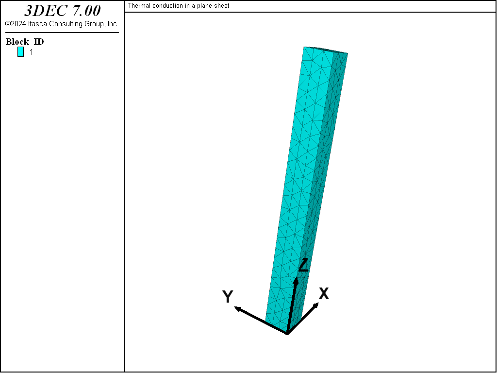
Figure 1: 3DEC grid for conduction in a plane sheet.
The example Conduction in a Plane Sheet — Explicit Solution contains the 3DEC data file for this problem. The comparison of analytical and numerical temperatures at three thermal times for the explicit solution is shown in Figure 2; the comparison for the implicit solution is shown in Figure 3. Normalized temperature (\(T/T\)1) is plotted versus normalized distance (\(z/L\)) in the two figures, where, Tables 2, 4, and 6 contain the analytical solution for temperatures, and Tables 1, 3, and 5 contain the 3DEC solutions. The three thermal times are 1.455, 7.273, and 72.73 seconds for the explicit solution, and 1.455, 11.45, and 71.45 seconds for the implicit solution. The solution has reached the equilibrium thermal state by the last time in each case. For both solution formulations, the difference between analytical and numerical temperatures at steady state is less than 0.1%.
Conduction in a Plane Sheet — Explicit Solution
; Thermal conduction in a plane sheet
; Compares explicit and implicit methods

model new
model random 10000
fish automatic-create off
model config thermal
model large-strain on
;
model title
Thermal conduction in a plane sheet
;

; --- fish constants ---
fish def cons
   global c_cond = 1.6             ; conductivity
   global c_dens = 1000.           ; density
   global c_sph = 0.2              ; specific heat
   global length = 1.              ; wall thickness
   global t1 = 100.                ; wall temperature, face 1
   global tabn = -1
   global tabe = 0
   global overl = 1. / length
   global d = c_cond / (c_dens * c_sph)
   global dol2 = d * overl * overl
   global top = 2. / math.pi
   global pi2 = math.pi * math.pi
   global n_max = 100              ; max number of terms -exact solution
   global teps = 1.e-5             ; small value compared to 1
end
[cons]

block create brick 0 0.1  0 0.1  0 [length]

block zone gen edgelength 0.04

block zone cmodel assign el
block zone prop dens [c_dens] bulk 6667 shear 4000

block contact material-table default prop stiffness-normal 1000 ...
                                          stiffness-shear 1000
;
block zone thermal prop cond [c_cond]  spec-heat [c_sph] exp 1e-5
;
block gridpoint apply temp [t1] range pos-z 0
block gridpoint apply temp 0 range pos-z 1
;
model hist thermal time-total ; or model his time-thermal
block hist temp pos 0 0 0
block hist temp pos 0 0 0.5
block hist temp pos 0 0 1
;
;block thermal list apply
;block gridpoint list therm
;

; for calculating analytical solution
program call "plane_sheet.fis"

model save 'psheet-ini'
;
; --- explicit method ---
model mechanical active off
model thermal active on
;
model cyc 20
[cons]
[num_sol]
[ana_sol]
model cyc 80
[num_sol]
[ana_sol]
model cyc 900
[num_sol]
[ana_sol]

table '1' label '3DEC 0.3 s'
table '2' label 'Analytical 0.3 s'
table '3' label '3DEC 1.5 s'
table '4' label 'Analytical 1.5'
table '5' label '3DEC 15 s'
table '6' label 'Analytical 15'

model save 'psheet-exp'

; -- implicit method ---
model restore 'psheet-ini'
model mechanical active off
block thermal implicit on
model mechanical timestep fix 1.e-1
model cyc 3
[num_sol]
[ana_sol]
model cyc 12
[num_sol]
[ana_sol]
model cyc 135
[num_sol]
[ana_sol]

table '1' label '3DEC 0.3 s'
table '2' label 'Analytical 0.3 s'
table '3' label '3DEC 1.5 s'
table '4' label 'Analytical 1.5'
table '5' label '3DEC 15 s'
table '6' label 'Analytical 15'

model save 'psheet-imp'
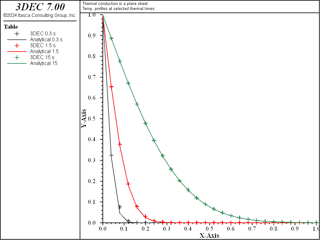
Figure 2: Comparison of temperatures for the explicit-solution algorithm (Tables 2, 4, and 6 = analytic solution; Tables 1, 3, and 5 = 3DEC solution).
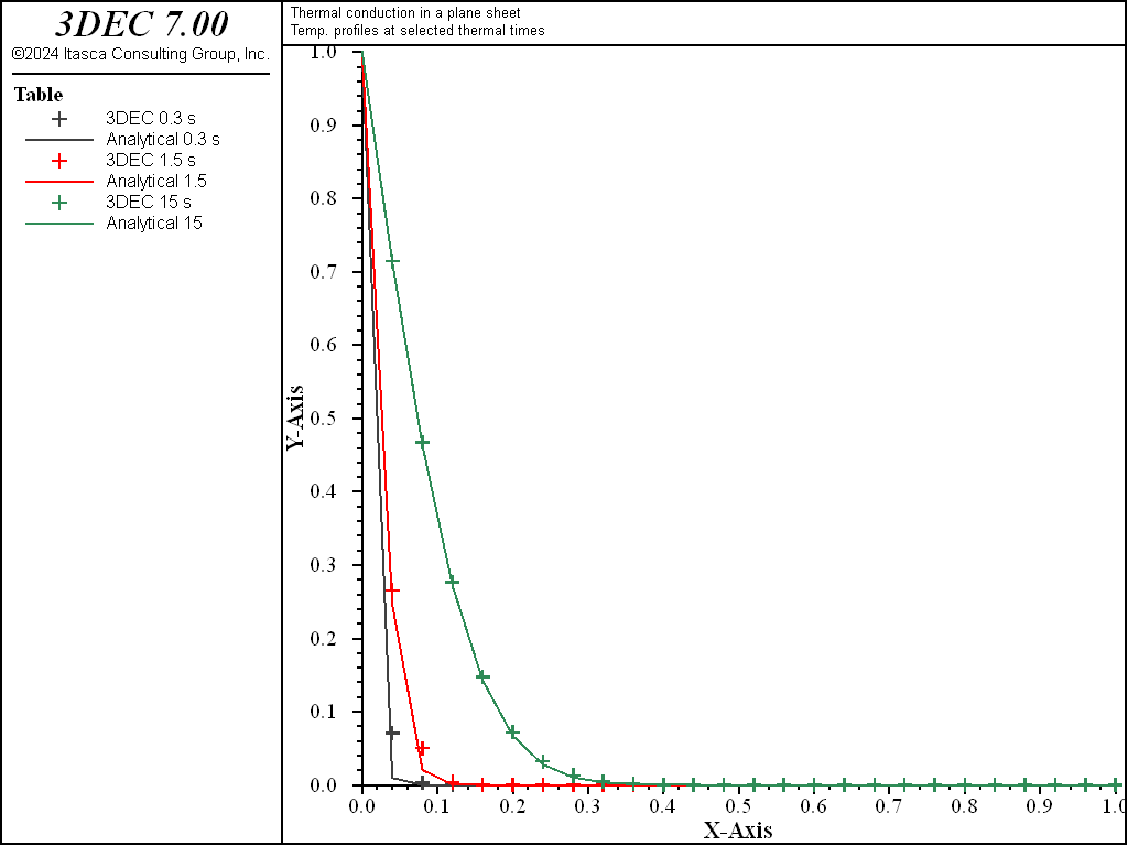
Figure 3: Comparison of temperatures for the implicit-solution algorithm (Tables 2, 4, and 6 = analytic solution; Tables 1, 3, and 5 = 3DEC solution).
Heating of a Hollow Cylinder
A hollow cylinder of infinite length is initially at a constant temperature of 0°C. The inner radius of the cylinder is exposed to a constant temperature of 100°C, and the outer radius is kept at 0°C. The problem is to determine the temperatures and thermally induced stresses in the cylinder when the equilibrium thermal state is reached.
Nowacki (1962) provides the solution to this problem in terms of the temperatures and radial, tangential and axial stresses at the steady-state thermal state:
where:
\(T\) = temperature;
\(r\) = radial distance from the cylinder center;
\(a\) = inner radius of the cylinder;
\(b\) = outer radius of the cylinder;
\(T_a\) = temperature at the inner radius;
\(\sigma_r\) = radial stress;
\(\sigma_t\) = tangential stress;
\(\sigma_a\) = axial stress;
\(m = {3 K \alpha_t \over {\lambda + 2 G}}\);
\(\lambda = K - {2 \over 3} G\);
\(K\) is the bulk modulus;
\(G\) is the shear modulus; and
\(\alpha_t\) is the linear thermal expansion coefficient.
The analytical solutions for temperature and stresses are programmed as FISH functions in the 3DEC data file. The analytical and numerical results can then be compared directly in tables.
The following properties are prescribed for this example:
Geometry
| inner radius of cylinder (\(a\)) | 1.0 m | |
| outer radius of cylinder (\(b\)) | 2.0 m | |
| Material Properties |
| density (\(\rho\)) | 2000 kg/m3 |
| specific heat (\(C_p\)) | 880.0 J/kg °C |
| thermal conductivity (\(k\)) | 4.2 W/m °C |
| linear thermal expansion coefficient (\(\alpha_t\) ) | 5.4 × 10⁻⁶/ °C |
| shear modulus (\(G\)) | 28.0 GPa |
| bulk modulus (\(K\)) | 48.0 GPa |
A thin quarter-section of the cylinder is modeled with 3DEC. Figure 4 shows the 3DEC grid. A constant-temperature boundary of 100°C is specified for the inner radius of the model; the temperature at the outer radius is specified to be 0°C.
The 3DEC model can be run as either an uncoupled or a coupled thermal-mechanical analysis. For a thermal-elastic analysis, it is more efficient to perform an uncoupled analysis. This is demonstrated by running both uncoupled and coupled models for this problem. We first run the model in an uncoupled mode: the thermal calculation is performed first to reach the equilibrium heat-flux state; then the thermally induced mechanical stresses are calculated. The 3DEC data file is listed in Heating of a Hollow Cylinder (“hollow-cyl.dat”).
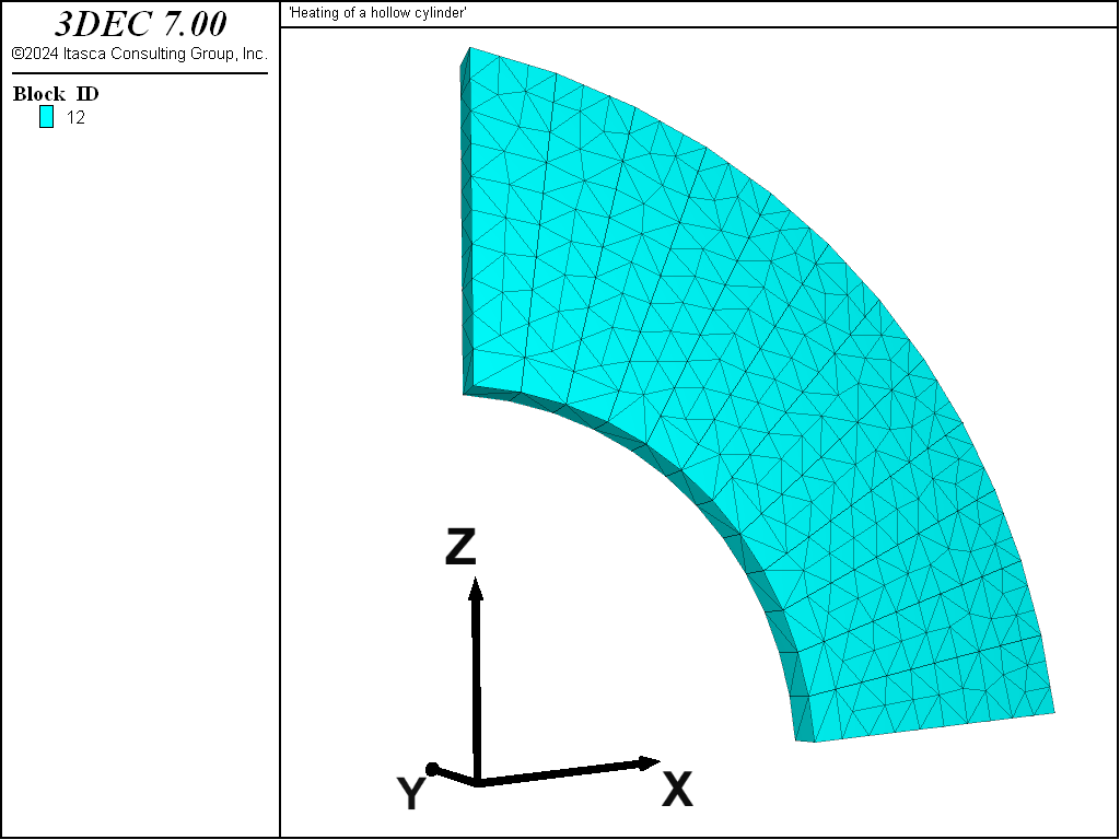
Figure 4: 3DEC grid for heating of a hollow cylinder.
Heating of a Hollow Cylinder (“hollow-cyl.dat”)
; ---------------------------------------------------------
; heating of a hollow cylinder
; ---------------------------------------------------------
model new
model random 10000
fish automatic-create off

model config thermal
model large-strain on

model title
'Heating of a hollow cylinder'

fish def cons
   global c_b = 2.0        ; radius
   global c_g = 28e9       ; shear modulus
   global c_k = 48e9       ; bulk  modulus
   global c_al = 5.4e-6    ; coefficient of thermal expansion
   global t1 = 100.        ; boundary temperature
   global oc1 = 1. / math.ln(c_b)
   global oc2 = 1. / (c_b * c_b - 1.)
   global oc3 = 0.5 * (c_k - c_g * 2. / 3.)/(c_k + c_g / 3.)
   global c_mmu = c_g * (3. * c_k * c_al) / (c_k + 4. * c_g / 3.)
   global tab1 = 1        ; numerical  temperature
   global tab2 = 2        ; analytical temperature
   global tab3 = 3        ; numerical  radial     stress
   global tab4 = 4        ; analytical radial     stress
   global tab5 = 5        ; numerical  tangential stress
   global tab6 = 6        ; analytical tangential stress
   global tab7 = 7        ; numerical  axial      stress
   global tab8 = 8        ; analytical axial      stress
end
[cons]
;
; create quarter-cylinder using prism blocks
fish def genb
  local xc = 0.0
  local zc = 0.0
  local ya = 0.0
  local yb = 0.1
  local dang = math.pi / (12.0 * 2.0)
  local dr = 0.1
  local ri = 1.0
  local re = c_b
  loop local i (1, 12)
    local ang = dang * float(i-1)
    local angn = dang * float(i)
    local rr = ri
    local rrn = re
    global x1 = xc + rr * math.cos(ang)
    global z1 = zc + rr * math.sin(ang)
    global x2 = xc + rrn * math.cos(ang)
    global z2 = zc + rrn * math.sin(ang)
    global x3 = xc + rrn * math.cos(angn)
    global z3 = zc + rrn * math.sin(angn)
    global x4 = xc + rr * math.cos(angn)
    global z4 = zc + rr * math.sin(angn)
    command
      block create prism &
        face-1 [x1] [ya] [z1] [x2] [ya] [z2] [x3] [ya] [z3] [x4] [ya] [z4] &
        face-2 [x1] [yb] [z1] [x2] [yb] [z2] [x3] [yb] [z3] [x4] [yb] [z4]
    endcommand
  endloop
end
[genb]

block join
;
; bug in quad that I can't find!
;block zone gen hex div 1 1 20 ; single_quad
block zone gen edgelength 0.1

block zone cmodel assign el
block zone prop dens 2000 bulk [c_k] shear [c_g]

block contact material-table default prop stiffness-normal 1000 ...
                                          stiffness-shear 1000
;
block zone thermal prop cond 4.2  spec-heat 880 exp [c_al]
;
block gridpoint apply vel-z 0.0 range pos-z 0
block gridpoint apply vel-x 0.0 range pos-x 0
block gridpoint apply vel-y 0.0 range pos-y 0
block gridpoint apply vel-y 0.0 range pos-y 0.1
;
block gridpoint apply temperature [t1] ...
                      range cyl end-1 0 -0.01 0 end-2 0 0.11 0 rad 0.99 1.01
block gridpoint apply temperature 0 ...
                      range cyl end-1 0 -0.01 0 end-2 0 0.11 0 rad 1.99 2.01

;
model his thermal time-total
block hist temp pos 1 0 0
block hist temp pos 1.5 0 0
block hist temp pos 2 0 0
block hist temp pos 0 0 1.5
block hist stress-zz pos  1 0 0
block hist stress-zz pos  1.5 0 0
block hist stress-zz pos  2 0 0
;
program call 'hollow-cyl.fis'
model save 'cyl-init'

;  uncoupled analysis
model mechanical active off
model thermal active on
model solve
;
model mechanical active on
model thermal active off
model solve ratio 1e-9

model thermal active on
[num_solt]
[ana_solt]
[num_solst]
[ana_solst]

table '1' label '3DEC Temperature'
table '2' label 'Analytical Temperature'
table '3' label '3DEC Radial Stress'
table '4' label 'Analytical Radial Stress'
table '5' label '3DEC Tangential Stress'
table '6' label 'Analytical Tangential Stress'
table '7' label '3DEC Axial Stress'
table '8' label 'Analytical Axial Stress'

model save 'cyl-ucpl'
;
;  coupled analysis
model restore 'cyl-init'
model mechanical active on
model thermal active on
model mechanical substep 100
model mechanical slave on

his int 10
model cyc 1000
model solve
[num_solt]
[ana_solt]
[num_solst]
[ana_solst]

table '1' label '3DEC Temperature'
table '2' label 'Analytical Temperature'
table '3' label '3DEC Radial Stress'
table '4' label 'Analytical Radial Stress'
table '5' label '3DEC Tangential Stress'
table '6' label 'Analytical Tangential Stress'
table '7' label '3DEC Axial Stress'
table '8' label 'Analytical Axial Stress'

model save 'cyl-cpl'
Numerical and analytical results are compared in Figure 5 and Figure 6. The figures show plots of tables for temperature and stress distributions through the cylinder at steady state. The plotted values are normalized: temperature is normalized by dividing by \(T_a\); and stress is normalized by dividing by \(mGT_a\). Figure 5 shows the temperature distribution at steady state for the numerical and analytical solutions. The agreement is very good, with an error of less than 0.1%. Acomparison of results for radial, tangential and axial stress distributions at steady state is provided in Figure 6.
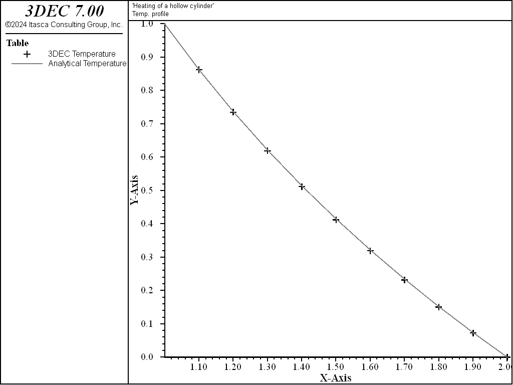
Figure 5: Temperature distribution at steady state for heating of a hollow cylinder.
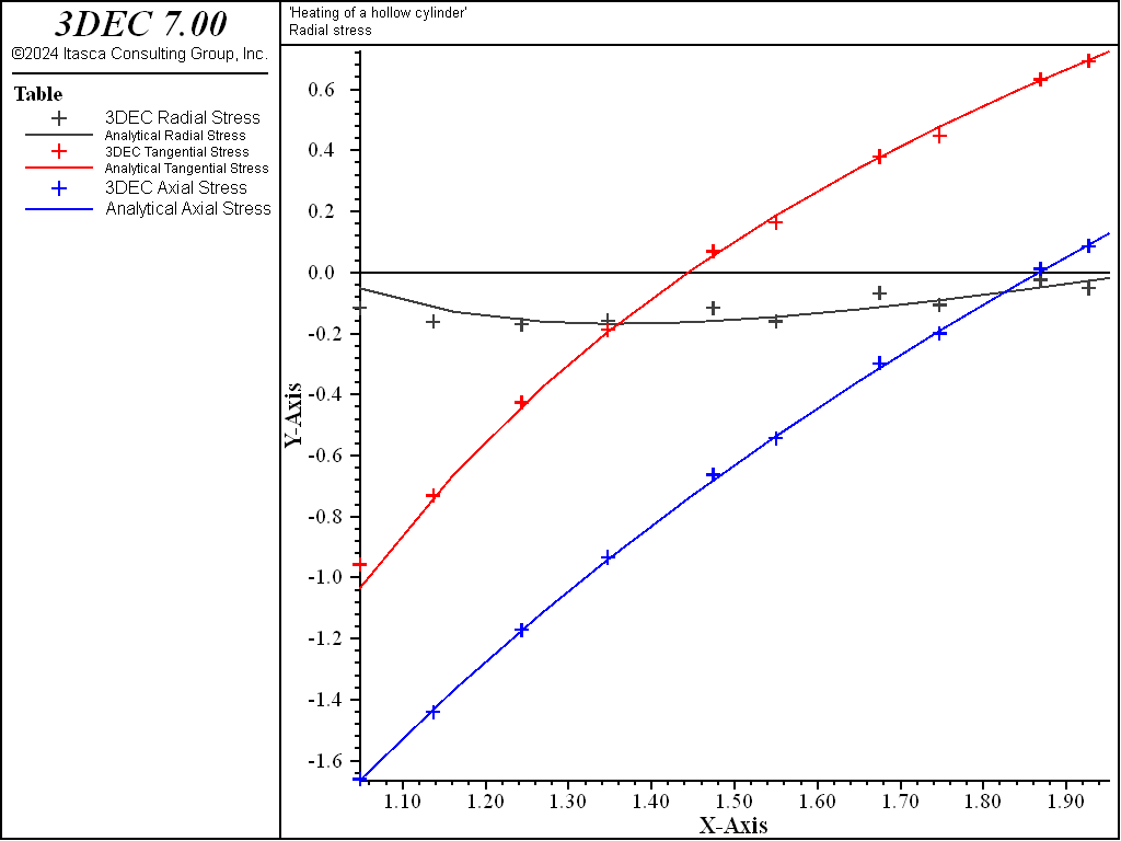
Figure 6: Radial stress distribution at steady state for heating of a hollow cylinder
Infinite Line Heat Source in an Infinite Medium
An infinite line heat source with a constant heat-generating rate is located in an infinite elastic medium with constant thermal properties. Nowacki (1962) provides the solution to this problem for the transient values of temperature, radial and tangential stress and radial displacement:
where:
\(\xi\) = {\({r^2}\over{4 \kappa t}\)};
\(r\) = radial distance to the line source;
\(\kappa\) = \(k \over {\rho C_p}\);
\(a\) = \({q \over {k}}\);
\(b\) = \(\alpha_t \ a {9 K \over {3K + 4G}}\);
\(L\) = unit length; and
\(E_1(\xi)\) = \(\int_{\xi}^\infty {e^{-u} \over {u}} du\) is the exponential integral.
The material properties and initial and boundary conditions for this example are defined:
Material Properties
| density (\(\rho\)) | 2000 kg/m3 |
| shear modulus (\(G\)) | 30 GPa |
| bulk modulus (\(K\)) | 50 GPa |
| specific heat (\(C_p\)) | 1000 J/kg °C |
| thermal conductivity (\(k\)) | 4 W/m °C |
| linear thermal expansion coefficient (\(\alpha t\)) | 5× 10⁻⁶/°C |
| Initial/Boundary Conditions |
| initial uniform temperature | 0°C | |
| initial stress state | no stresses | |
| Line Heat Source |
| energy release per unit length (\(q\)) | 1600 W/m |
It is assumed that the material properties are temperature-independent, the thermal output of the source is constant (no decay), and the line heat source is of infinite length.
The 3DEC grid for this problem is a radial sector of \(1 \over 192\) of a cylindrical disk. The axis of the line heat source coincides with the \(y\)-axis of the model. The grid is radially graded in the \(xz\)-plane; a single layer of zones is used in the \(y\)-direction. The model is shown in Figure 7. A FISH function (fxface.fis) is used to apply the roller boundaries at the inclined boundary.
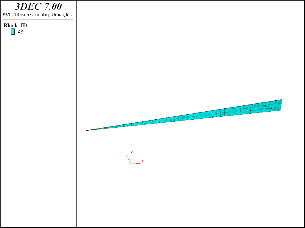
Figure 7: 3DEC model for an infinite line heat source.
The line heat source is represented in 3DEC by a series of point sources. The intensity of the point-source strength, \(q_p\), is adjusted to produce an equivalent intensity to the line heat source, \(Q\). For a quarter-symmetry model and one zone thickness, the relation between \(q_p\) and \(Q\) is
where \(L\) = length of the line source represented in the model.
The constant heat source is applied at the gridpoints along the \(y\)-axis; the boundaries of the model are kept adiabatic to represent thermal symmetry planes. The grid is extended to a distance of 500 m from the \(y\)-axis to simulate infinity. The far boundary is mechanically fixed; the boundaries along the \(x\)-axis and \(z\)-axis are fixed to represent shear-free symmetry planes.
An uncoupled analysis is recommended because the material is elastic. The problem is first thermally solved to an age of one year (model mechanical active off) using the implicit-solution algorithm, and then stepped to mechanical equilibrium (model thermal active off and model mechanical active on). The heat source produces uniform motion in one direction for this problem. This case is better-suited to combined damping than local damping (see the topic “Mechanical Damping” in 3DEC Theory and Background). The 3DEC data file is listed in “Infinite line heat source in an infinite medium.”
The dimensionless form of the analytical solutions in Equation (61) through Equation (64) is programmed as FISH functions in the example “Infinite line heat source in an infinite medium.” The analytical and numerical values can then be compared directly in tables. The analytical solutions for temperature and radial displacement are programmed in the FISH function fana�_soltu, and for radial and tangential stresses in fana�_solst. The exponential integral function used in the analytical solutions is programmed as a separate FISH function contained in file “EXP_INT.FIS”. The dimensionless values for the numerical results for temperature and displacement are calculated in the FISH function fnum�_soltu, and for radial and tangential stresses in fnum�_solst. The numerical values for dimensionless temperature, radial stress, tangential stress and radial displacement are stored in Tables 1, 3, 5, and 7, respectively. The analytical values for dimensionless temperature, radial stress, tangential stress and radial displacement are stored in Tables 2, 4, 6, and 8, respectively.
The results for temperature, radial displacement and radial and tangential stress distributions at 1 year are presented in the table plots in Figure 8 through Figure 10. The difference between numerical and analytical solutions for temperature is less than 2%. The comparison is also good for displacements and for stresses; the difference is generally less than 2% within 100 m of the heat source. The fixed outer boundary has an influence on the numerical results further from the source, but the agreement is still reasonable.

Figure 8: Temperature distribution at 1 year.
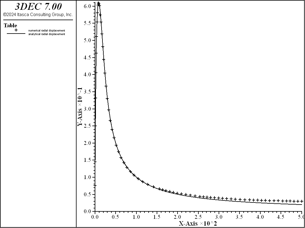
Figure 9: Radial displacement distribution at 1 year.
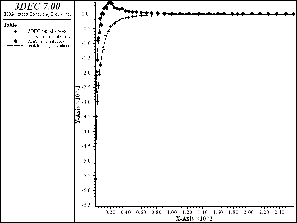
Figure 10: Radial and tangential stress distributions at 1 year.
Infinite line heat source in an infinite medium
; ---------------------------------------------------------
; infinite line source in an infinite medium
;
; ---------------------------------------------------------
model new
fish automatic-create off
model config thermal
model large-strain on

model title 'Infinite line heat source in infinite elastic medium'

block tolerance 0.001

fish def gcons           ; geometrical constants
   global n1 = 48
   global n2 = 24
   global y1 = 1.
end
[gcons]

fish def cons
   global c_g = 3.e10         ; shear modulus
   global c_k = 5.e10         ; bulk  modulus
   global c_al = 5.e-6        ; coefficient of thermal expansion
   global t1 = 100.0          ; boundary temperature
   global c_tk = 4.           ; conductivity
   global c_cp = 1e3          ; specific heat
   global q_q  = 1600.        ; line source intensity
   global c_density = 2.e3
   local kappa = c_tk / (c_density * c_cp)
   global o4c = 1. / (4. * kappa)
   global o4p = 1. / (4. * math.pi)
   global o8p = o4p * 0.5
   local val = c_k / c_g
   global c_nu = (3.*val-2.)/(6.*val+2.)
   global c_eta = c_al * c_g * (1.+c_nu)/(1.-c_nu)
   global a_a = q_q / c_tk
   global b_b = c_eta * a_a
   global c_c = b_b * 1.0 / c_g
   a_a = 1. / a_a
   b_b = 1. / b_b
   c_c = 1. / c_c
   global tab1 = 1        ; numerical  temperature
   global tab2 = 2        ; analytical temperature
   global tab3 = 3        ; numerical  radial     stress
   global tab4 = 4        ; analytical radial     stress
   global tab5 = 5        ; numerical  tangential stress
   global tab6 = 6        ; analytical tangential stress
   global tab7 = 7        ; numerical  radial     displacement
   global tab8 = 8        ; analytical radial     displacement
   global tab11 = 11        ; numerical  temperature (x<100)
   global tab12 = 12        ; analytical temperature (x<100)
end
[cons]

; ---- create geometry -----
fish def genb
  local xc = 0.0
  local zc = 0.0
  local ya = 0.0
  local yb = y1
  global dang = math.pi / (float(n2) * 2.0)
;
  local rr = 1.0
  local dr = 1.0
  loop local i (2,n1)
    dr = dr * 1.1
    rr = rr + dr
  endloop
  local dr1 = 500.0 / rr
;
  local rrn = 0.0
  dr = dr1
  loop i (1, n1)
    local i1 = i
    local ang = 0.0
    local angn = dang

    rr = rrn
    if i > 1
      dr = dr * 1.1
    endif
    rrn = rr + dr
    global  x1 = xc + rr * math.cos(ang)
    global  z1 = zc + rr * math.sin(ang)
    global  x2 = xc + rrn * math.cos(ang)
    global  z2 = zc + rrn * math.sin(ang)
    global  x3 = xc + rrn * math.cos(angn)
    global  z3 = zc + rrn * math.sin(angn)
    global  x4 = xc + rr * math.cos(angn)
    global  z4 = zc + rr * math.sin(angn)
    if i = 1
        command
          block create prism &
            face-1 [x1] [ya] [z1]  [x2] [ya] [z2]  [x3] [ya] [z3] &
            face-2 [x1] [yb] [z1]  [x2] [yb] [z2]  [x3] [yb] [z3]
        endcommand
    else
        command
          block create  prism &
            face-1 [x1] [ya] [z1]  [x2] [ya] [z2]  ...
                   [x3] [ya] [z3]  [x4] [ya] [z4]  ...
            face-2 [x1] [yb] [z1]  [x2] [yb] [z2]  ...
                   [x3] [yb] [z3]  [x4] [yb] [z4]
        endcommand
    endif
  endloop
end
[genb]

; split block to refine mesh near source
block cut joint-set dip 90 dip-direction 90 or 0.25 0.0 0.0
block join

block zone gen edgelength 10

block zone cmodel assign el
block zone prop dens [c_density] bulk [c_k] shear [c_g]
;
block contact material-table default prop stiffness-normal 1000 ...
                                          stiffness-shear 1000
;
block zone thermal prop cond [c_tk] spec-heat [c_cp] exp [c_al]
;
block gridpoint apply vel-z 0 range pos-z 0
block gridpoint apply vel-x 0 range pos-x 0
block gridpoint apply vel-y 0 range pos-y 0
block gridpoint apply vel-y 0 range pos-y 1
;
; point source strength for 1/48 of quarter space
fish def ppp
  ppp = 1600.0 * 0.5 / (float(n2) * 4.0)
end

block gridpoint apply source [ppp] range pos-x 0
;
model hist thermal time-total ; or model his time-thermal
block hist temp pos 0 0 0
block hist temp pos 1 0 0
block hist temp pos 5 0 0
block hist temp pos 10 0 0
block hist temp pos 500 0 0
block hist dis-x pos 1 0 0
block hist dis-x pos 10 0 0
block hist dis-x pos 100 0 0
block his stress-xx pos 1 0 0
block his stress-xx pos 10 0 0
block his stress-xx pos 100 0 0

;  uncoupled analysis (implicit)
model mechanical active off
model thermal active on
block thermal implicit on

model thermal timestep fix 500
model step 63000

model save 'ils_year0'

; apply roller boundaries on plane at angle DANG
block face apply vel-norm 0 ...
      range plane dip [dang/math.degrad] d-d 270 dist 1e-3 pos-x 0.1 500


model mechanical active on
model thermal active off
block mech damp combined
model step 40000
model save 'ils_year1'

program call "solution.fis"
[num_soltu]
[ana_soltu]
[num_solst]
[ana_solst]

table '1' label '3DEC temperature'
table '2' label 'analytical temperature'
table '3' label '3DEC radial stress'
table '4' label 'analytical radial stress'
table '5' label '3DEC tangential stress'
table '6' label 'analytical tangential stress'
table '7' label 'numerical radial displacement'
table '8' label 'analytical radial displacement'
table '11' label '3DEC temperature (radius<100)'
table '12' label 'analytical temperature (radius<100)'

model save "ils_solution"
FISH function – “solution.fis”
;
; analytical and numerical solutions for infinite line heat source problem
;
program call "exp_int.fis"
fish def num_soltu
;
; INPUT: tab1 - table of numerical temperatures
;        tab7 - table of numerical radial displacements
;        tab11 - table of numerical temperature (radius < 100)
;
  global nn = 0
  loop foreach local gp_ block.gp.list
      local rad = math.sqrt(block.gp.pos.y(gp_)^2 + block.gp.pos.z(gp_)^2)
      if rad < 1.e-4 then
         local x = block.gp.pos.x(gp_)
         if x > 1.0e-4
           table(tab1,x) = block.gp.temp(gp_) * a_a
           nn = nn + 1
           if x < 100.0
             table(tab11,x) = table(tab1,x)
           endif
         endif
         table(tab7,x) = block.gp.disp.x(gp_) * c_c
      end_if
  end_loop
  nn = 48
end
;
fish def ana_soltu
;
; INPUT: tab2 - table of analytical temperatures
;        tab8 - table of analytical radial displacements
;        tab12 - table of analytical temperature (radius < 100)
;
  loop foreach local gp_ block.gp.list
      local rad = math.sqrt(block.gp.pos.y(gp_)^2 + block.gp.pos.z(gp_)^2)
      if rad < 1.e-4 then
         local x = block.gp.pos.x(gp_)
         if x = 0.0 then
           table(tab2,x) = 0.0
           table(tab8,x) = 0.0
         else
           local e_val = x * x * o4c / thermal.time.total
           local val = exp_int(e_val)
           table(tab2,x) = val * o4p
           table(tab8,x) = (val + (1.-math.exp(-e_val))/e_val) * x * o8p
           if x < 100.0
             table(tab12,x) = table(tab2,x)
           endif
         end_if
      end_if
  end_loop
end
;
fish def num_solst
;
; INPUT: tab3 - table of numerical radial stress
;        tab5 - table of numerical tangential stress
;
   local ns = 1
   loop while ns < nn
      local x = (table.x(tab1,ns) + table.x(tab1,ns+1)) * 0.5
      local p_z = block.zone.near(x,0.,0.)
      local xc = block.zone.pos.x(p_z)
      local zc = block.zone.pos.z(p_z)
      local ra2 = xc*xc + zc*zc
      if ra2 # 0
        local ra = math.sqrt(ra2)
        table.x(tab3,ns) = ra
        local zstress = block.zone.stress(p_z)
        local val = (zstress->xx*xc*xc + zstress->zz*zc*zc + ...
                                         2.*zstress->xz*xc*zc)/ra2
        table.y(tab3,ns) = val * b_b
        table.x(tab5,ns) = ra
        val = (zstress->xx*zc*zc + zstress->zz*xc*xc - ...
                                   2.*zstress->xz*xc*zc)/ra2
        table.y(tab5,ns) = val * b_b
      endif
      ns = ns + 1
   end_loop
end

fish def ana_solst
;
; INPUT: tab4 - table of analytical radial stress
;        tab6 - table of analytical tangential stress
;
   local ns = 1
   loop while ns < nn
      local x = (table.x(tab1,ns) + table.x(tab1,ns+1)) * 0.5
      if x # 0
        local p_z = block.zone.near(x,0.,0.)
        local xc = block.zone.pos.x(p_z)
        local zc = block.zone.pos.z(p_z)
        local ra2 = xc*xc + zc*zc
        if ra2 # 0
          local ra = math.sqrt(ra2)
          local e_val = ra2 * o4c / thermal.time.total
          local val1 = exp_int(e_val)
          if e_val # 0
            local val2 = (1. - math.exp(-e_val)) / e_val
            table.x(tab4,ns) = ra
            table.y(tab4,ns) = - (val1 + val2) * o4p
            table.x(tab6,ns) = ra
            table.y(tab6,ns) = - (val1 - val2) * o4p
          endif
        endif
      endif
      ns = ns + 1
   end_loop
end
One-Dimensional Thermal Transport by Conduction and Convection
This validation problem illustrates the effect of forward and backward convection, at steady-state, on the conduction temperature profile in a saturated plane sheet. The saturated sheet has thickness a, and length L, and is modeled in 3DEC by a horizontal fracture of aperture \(a\). The fracture is located in a block that is kept adiabatic for the simulation. A system of axes is defined, with the \(x\)-axis pointing to the right along the fracture plane, and the origin located on the left boundary of the model. The temperature boundary conditions correspond to fixed temperatures: \(T\)1 at \(x\) = 0, and \(T\)2 at \(x\) = L. There is a constant fluid flux in the sheet, corresponding to a fixed boundary pressure \(P\)1 to the left, and \(P\)2 to the right of the model.
At steady state, the one-dimensional form of the energy balance equation may be expressed as
where \(\hat T = (T - T_1)/T_1, \hat x = x/L\), and \(P_e\) is the problem Peclet number. The Peclet number is defined as
where \(\rho_f\) is fluid density, \(C_f\) is fluid specific heat, \(q\) is fluid specific discharge, and \(k^T_f\) is fluid thermal conductivity. The specific discharge is given by the formula
where \(\mu\) is fluid viscosity.
The solution (with boundary conditions \(\hat T\) = 0 at \(\hat x\) = 0, and \(\hat T = \hat T_2\) at \(\hat x\) = 1) is
The values for the model properties and parameters are listed below.
| \(\rho_f\) | 1000 kg/m3 |
| \(C_f\) | 4200 J/kg/C |
| \(k^T_f\) | 0.6 W/m/C |
| \(\mu\) | 10−3 Pa.sec |
| \(a\) | 10−4 m |
| \(L\) | 4 m |
| \(T\)1 | 150 C |
| \(T\)2 | 130 C |
| \(P\)1 | Case 1: 0.2 Pa. Case 2: 0 Pa. |
| \(P\)2 | Case 1: 0 Pa. Case 2: 0.2 Pa. |
The Peclet number for the simulation has a magnitude of 1.17. The thermal flux is oriented to the right. Two simulations are carried out: case 1 is for convection and conduction acting in the same direction (flow to the right); and case 2 for flow to the left (convection and conduction acting in opposite directions). The 3DEC temperature profile for steady-state conduction-convection is compared to the analytical solution in Figure 11 and Figure 12. As may be seen from these figures, the match is very good for this particular simulation. The steady-state conduction solution (straight line) is also sketched on the plots. Compared to the conduction solution, the effect of fluid flow is seen to displace the temperature curves in the direction of the flow.
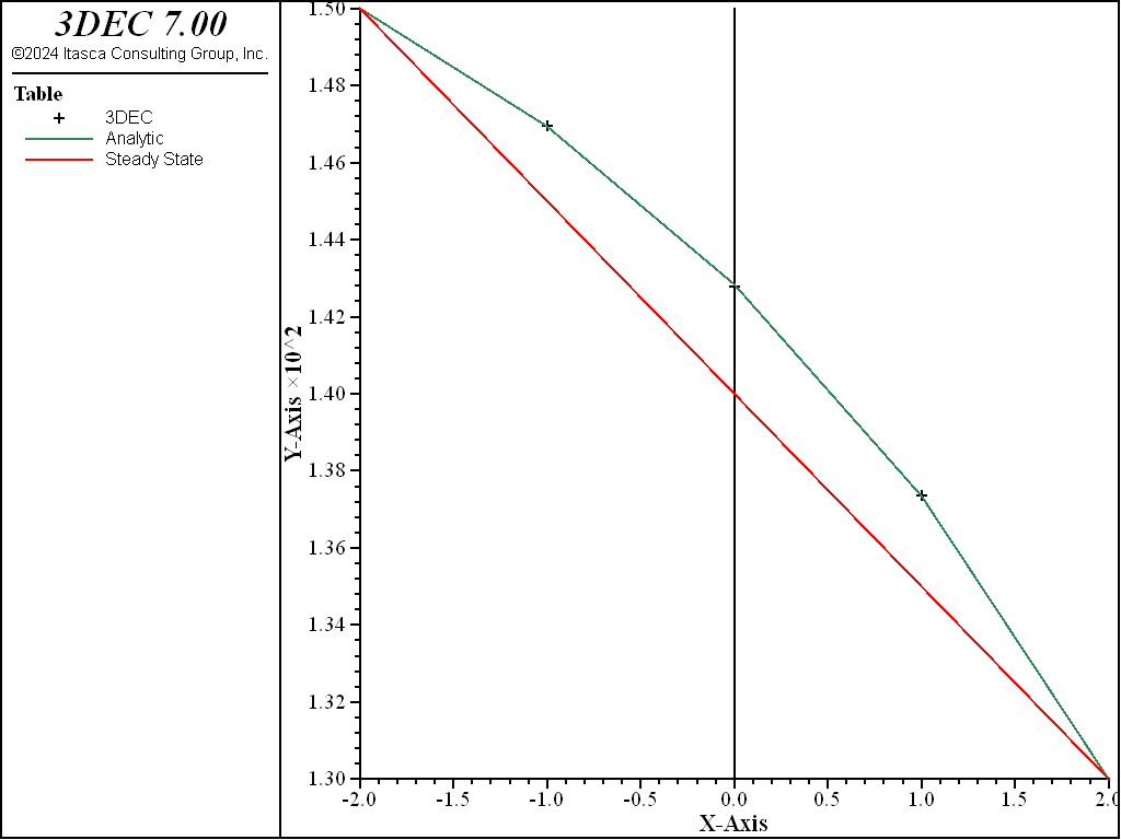
Figure 11: Analytical and numerical temperature profiles, compared to conduction solution at steady state — case 1.
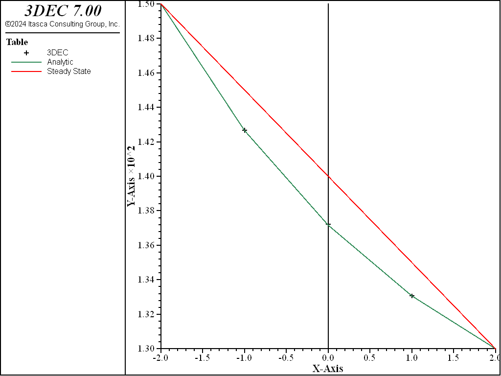
Figure 12: Analytical and numerical temperature profiles, compared to conduction solution at steady state — case 2.
convection_conduction.dat
; convection left to right

model new
model title
  'Conduction/advection in a fracture'
model config thermal fluid
model large-strain off

fish def setup
  _rhow = 1000
  _cw   = 4200.0
  _kt   = 0.6
  _visc = 1e-3
  _a    = 1e-4
  _x1   = -2.0
  _x2   =  2.0
  _t1   = 150.0
  _t2   = 130.0
  _right = 1
; for flow to the left set _right = 0
; _right = 0
  if _right = 1 then
    _p1   = 0.2
    _p2   = 0.0
  else
    _p1   = 0.0
    _p2   = 0.2
  endif
; --- for no flow (no convection), use:
; _p1   = 0.0
; _p2   = 0.0
;
  _L    = _x2 - _x1
  _perm = _a^2/(12.0*_visc)
  _q    = -_perm*(_p2-_p1)/_L
  _Pe   = _rhow*_cw*_q*_L/_kt
end
[setup]
;
block create brick [_x1] [_x2] -1 1 -1 1
block cut joint-set dip 0 dip-direction 0
;
block zone generate edgelength 1.0
;
flowplane vertex prop ap-ini=[_a] ap-min=1e-5 ap-max=1e-3
block fluid property bulk=2e9 density=[_rhow] visc=[_visc]
; --- model new fluid properties ---
block fluid property specific-heat=[_cw] thermal-conductivity=[_kt] ...
                     heat-transfer-coefficient=0

block zone cmodel assign el
block zone prop dens 1400 bulk 6e9 shear 4e9
block zone thermal prop expansion 1.0e-5 conductivity 0.2  specific-heat 800

block contact jmodel assign el
block contact prop stiffness-normal 1e9 stiffness-shear 1e9

;
model hist thermal time-total
block hist temp pos -2 1 1
block hist temp pos 0 1 1
block hist temp pos 0 -1 -1
block hist temp pos 2 1 1

; --- initial and boundary thermal conditions for the fluid ---
flowknot initialize temp [_t2]
flowknot apply temp [_t2] range pos-x  2.0
flowknot apply temp [_t1] range pos-x -2.0
; --- establish steady state flow field ---
block insitu p-p 0
flowknot apply p-p [_p2] range pos-x  2.0
flowknot apply p-p [_p1] range pos-x -2.0
model mechanical active off
model thermal active off
model fluid active on
model cycle 1000

; --- run the thermal simulation ---
block thermal convection on
model mechanical active off
model thermal active on
model fluid active off
model cyc 1000
model save 'adv'

; --- check results ---
fish def _ftemp
  loop foreach pnt flowknot.list
    _y = flowknot.pos.y(pnt)
    if _y < -0.99 then
      _x = flowknot.pos.x(pnt)
      _t = flowknot.temp(pnt)
      table(10,_x) = _t
      _xhat = (_x+2.0)/_L
      if _p1 = _p2 then
        term = _xhat
      else
        term = (math.exp(_Pe*_xhat)-1.0)/(math.exp(_Pe)-1.0)
      endif
      _anat = _t1+(_t2-_t1)*term
      table(11,_x) = _anat
      table(12,_x) = _t1+(_t2-_t1)*_xhat
    end_if
  end_loop
end
[_ftemp]
table '10' label '3DEC'
table '11' label 'Analytic'
table '12' label 'Steady State'
model title
  '1D conduction/convection'
The stability of the numerical convection algorithm implemented in 3DEC can be appreciated by exercising the data file for various values of the grid Peclet and Courant numbers. For example, by varying grid density and specific discharge, the values of grid Peclet and Courant numbers for which the algorithm is stable may be derived (see the Stability and Accuracy section describing numerical stability).
Application Examples
Thermal Convection in a Fracture at Depth
The 3DEC thermal-fluid coupling algorithm was used to analyze thermal conduction and convection in a single fracture at depth.
The properties were
| Rock | ||
| Density | 2700 kg/m3 | |
| Bulk modulus | 6 × 10⁹ Pa | |
| Shear modulus | 4 × 10⁹ Pa | |
| Thermal conductivity | 2.8 W/m/°C | |
| Specific heat | 800 J/kg/°C | |
| Fracture | ||
| Normal stiffness | 1 × 10⁹ Pa/m | |
| Shear stiffness | 1 × 10⁹ Pa/m | |
| Aperture | 2 × 10⁻⁵ m | |
| Fluid | ||
| Density | 1000 kg/m3 | |
| Bulk modulus | 2 × 10⁹ Pa | |
| Viscosity | 1 × 10⁻³ Pa.sec | |
| Thermal conductivity | 0.6 W/m/°C | |
| Specific heat | 4200 J/kg/°C |
Fluid-rock heat transfer coefficient 1, 10, 100 W/m2/°C.
The in-situ conditions, intended to simulate a depth of 4500-5000 m, were
| Vertical stress | 10 × 106 Pa | |
| Fluid pressure | 5 × 10⁶ Pa | |
| Rock temperature | 190 °C | |
| Fluid temperature | 190 °C |
A cubic domain of 0.5 × 0.5 × 0.5 m was modeled, with the fracture placed on the plane at \(y\) = 0. The block geometry is shown in Figure 13, and the block discretization in Figure 14.
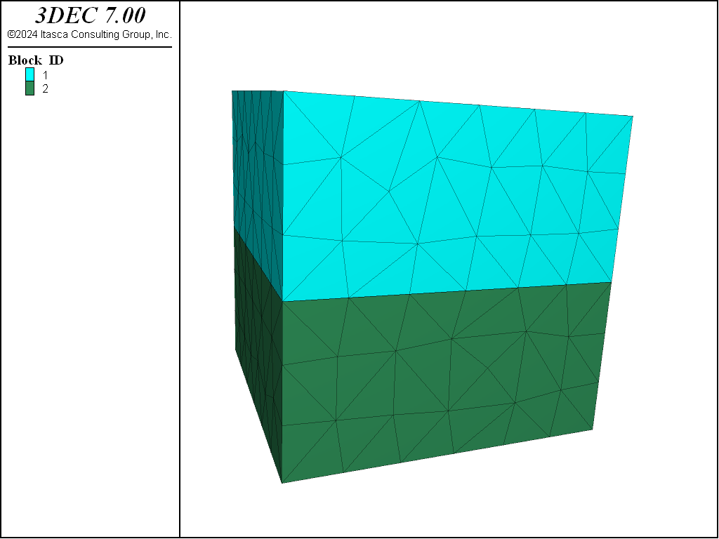
Figure 13: 3DEC block geometry for thermal convection in a fracture.
In the first stage, the in-situ conditions were applied without fluid flow or temperature gradients. In the second stage, fluid flow at the in-situ temperature was simulated by applying an inflow into the fracture of 2 × 10⁻⁷ m3/s/m at the boundary \(x\) = −0.25 m, and an equal outflow at the boundary \(x\) = 0.25 m. These boundary conditions produced a uniform flow velocity of 0.01 m/s in the fracture, and a fluid pressure distribution; both are shown in Figure 14.
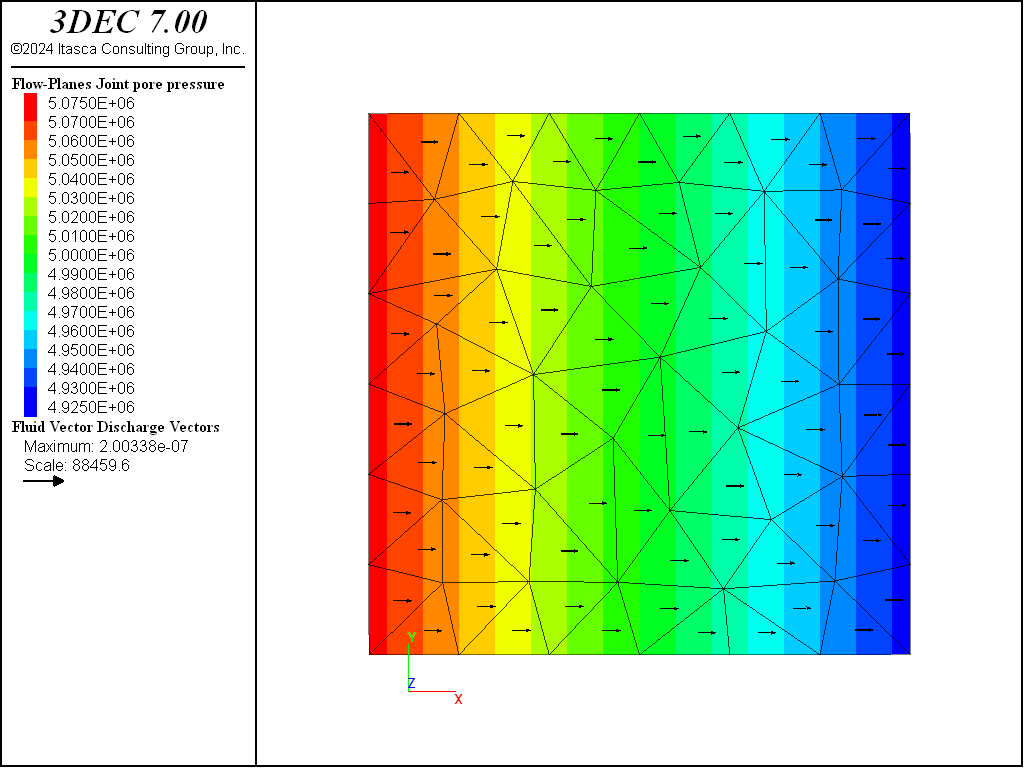
Figure 14: Flow velocity and fluid pressure distribution in the fracture.
In the third stage, the injection fluid temperature was fixed at 50°C at the boundary \(x\) = −0.25 m. At the outflow boundary, the fluid temperature was left free. The rock temperature was fixed at 190°C on all of the model outer boundaries.
Three values were considered for the heat transfer coefficient, \(h\):
- Case 1: \(h\) = 1 W/m2/°C
In this case, the fluid temperature is progressively reduced along the fracture, reaching a value of about 150°C at the outflow boundary. The final distribution of fluid temperatures is shown in Figure 15.
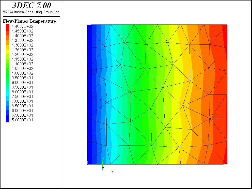
Figure 15: Fluid temperature contours at steady state — case 1.
The history of fluid temperature at 5 points along the fracture is presented in Figure 16. The rock temperature histories at 3 locations along the fracture are shown in Figure 17 (on a different time scale). The maximum drop of rock temperature is about 4°C near the center of the joint, as the rock temperature is kept fixed at 190°C on the model boundaries, including the fluid outflow boundary at \(x\) = 0.25 m.
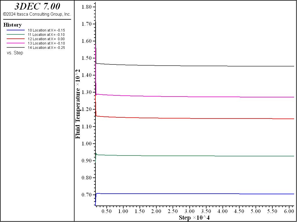
Figure 16: History of fluid temperature at 5 monitoring points — case 1.
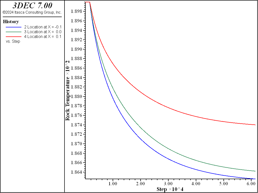
Figure 17: History of rock temperature at 3 monitoring points — case 1.
- Case 2: \(h\) = 10 W/m2/°C
For this value of the heat transfer coefficient, the heat flux from the rock to the fluid is higher. The fluid temperature approaches the rock temperature of 190°C a short distance from the inflow boundary. The final distribution of fluid temperatures is shown in Figure 18.
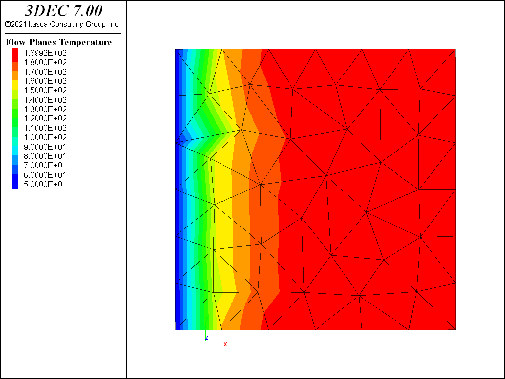
Figure 18: Fluid temperature contours at steady state — case 2.
The history of fluid temperature at the same 5 points along the fracture is presented in Figure 19. The rock temperature histories at 3 locations along the fracture are plotted in Figure 20.
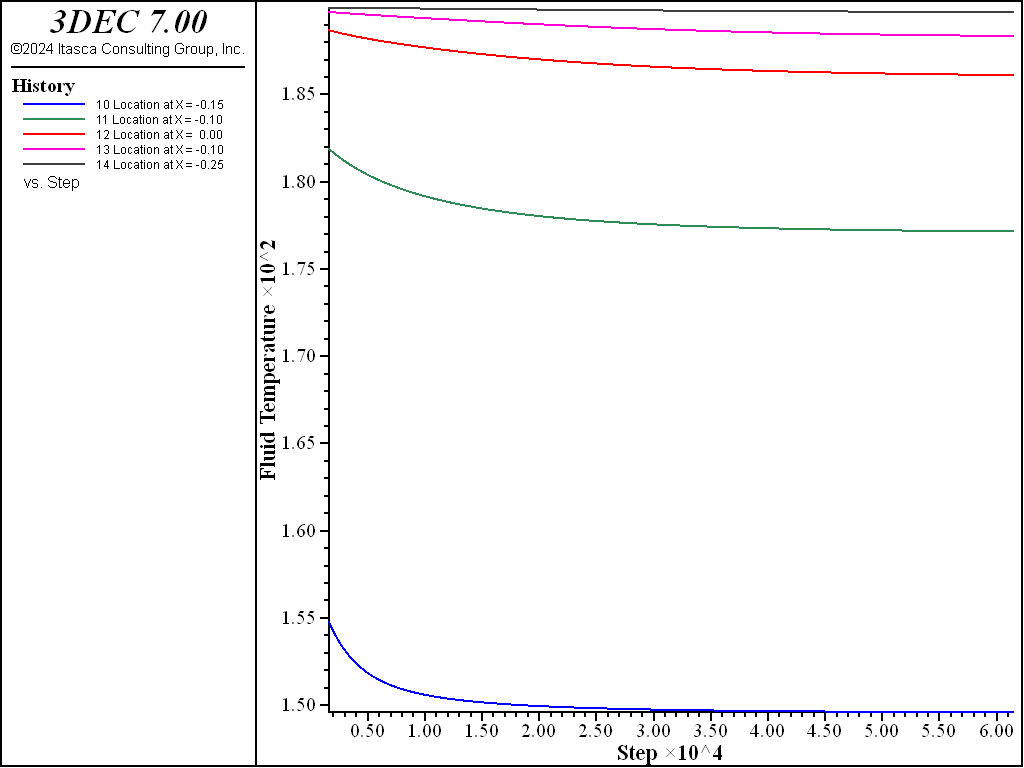
Figure 19: History of fluid temperature at 5 monitoring points — case 2.
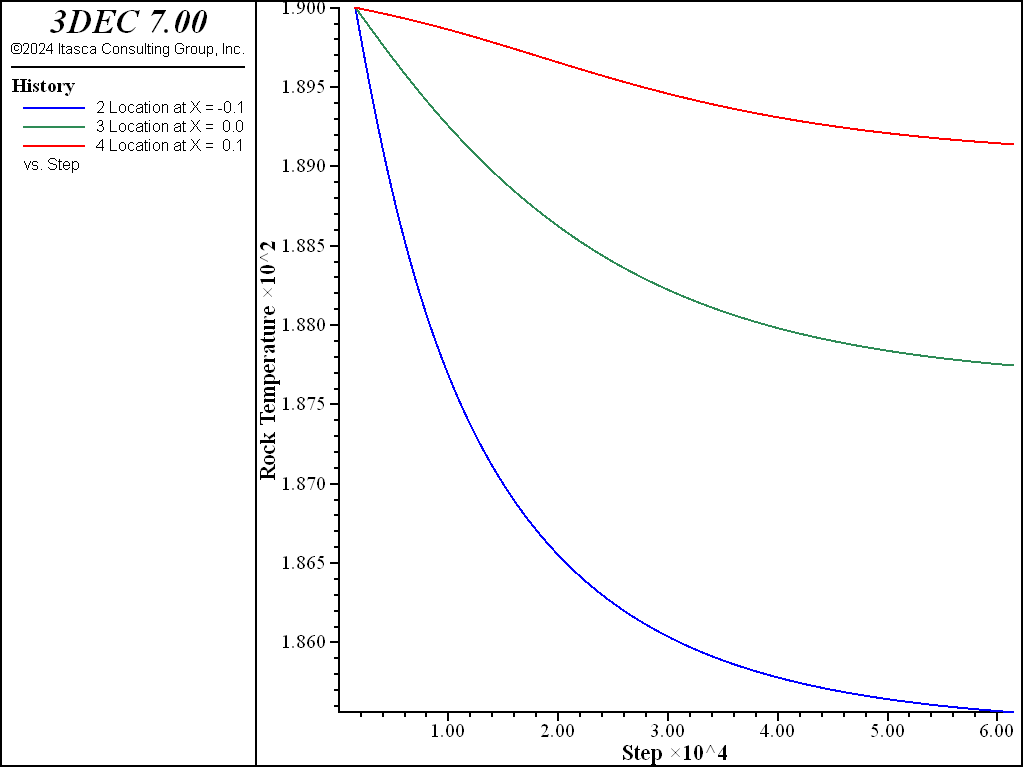
Figure 20: History of rock temperature at 3 monitoring points — case 2.
- Case 3: \(h\) = 100 W/m2/°C
The larger value of the heat transfer coefficient increases the heat flux from the rock to the fluid. The fluid temperature approaches the rock temperature of 190°C more rapidly than in the previous case. The final distribution of fluid temperatures is shown in Figure 21.
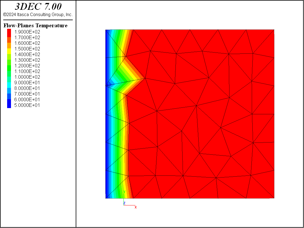
Figure 21: Fluid temperature contours at steady state — case 3.
The history of fluid temperature at 5 points along the fracture is presented in Figure 22, and the rock temperature histories at 3 locations are presented in Figure 23. (Note that the rock temperature is kept at 190°C on all model boundaries.)
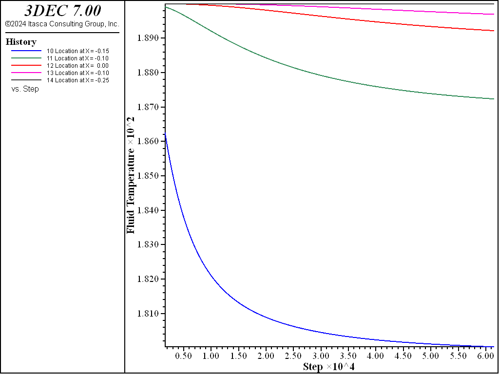
Figure 22: History of fluid temperature at 5 monitoring points — case 3.
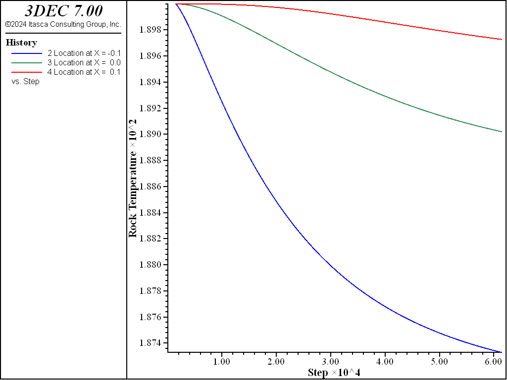
Figure 23: History of rock temperature at 3 monitoring points — case 3.
Data File
model new
; ---------------------------------------------------------
; 2 block test, fluid/rock heat transfer
; domain : 5.00x5.00x5.00 m
; depth : z=0 corresponds to a depth of 4750 m
; ---------------------------------------------------------
model config thermal fluid
model large-strain off

;
block create brick -0.250 0.250 -0.250 0.250 -0.250 0.250

block cut joint-set dip 0 dip-direction 0  or 0 0 0

block zone generate edgelength 0.08
;
; joint/fluid properties
flowplane vertex property aperture-initial 1e-4 ...
                          aperture-minimum 2e-5 aperture-maximum 1e-3
block fluid property bulk 2e9
block fluid property density 1000
block fluid property viscosity 1e-3
; --- fluid thermal properties ---
block fluid property specific-heat 4200.0
block fluid property thermal-conductivity 0.6
block fluid property heat-transfer-coefficient 10
;
;
;
; rock properties
block zone cmodel assign elastic
block zone property density 2700 bulk 6e9 shear 4e9
block zone thermal property expansion 1.0e-5 ...
                            conductivity 2.8 specific-heat 800

block contact jmodel assign mohr
block contact property stiffness-normal 1e9 stiffness-shear 1e9
;
; --- rock temperature : initial and boundary conditions ---
block gridpoint initialize temperature 190
block gridpoint apply temperature 190 range position-x -0.25
block gridpoint apply temperature 190 range position-x 0.25
block gridpoint apply temperature 190 range position-y -0.25
block gridpoint apply temperature 190 range position-y 0.25
block gridpoint apply temperature 190 range position-z -0.25
block gridpoint apply temperature 190 range position-z 0.25
;
; --- intial fluid temperature ---
block insitu fluid-temp 190

; --- insitu stresses and fluid pp ---
block insitu stress 0 0 -10e6 0 0 0
block insitu pore-pressure 5e6
; --- mechanical boundary conditions ---
block face apply stress 0 0 -10e6 0 0 0 range position-z .24 .26
block gridpoint apply velocity-x 0 range position-x -0.25
block gridpoint apply velocity-x 0 range position-x 0.25
block gridpoint apply velocity-y 0 range position-y -0.25
block gridpoint apply velocity-y 0 range position-y 0.25
block gridpoint apply velocity-z 0 range position-z -0.25
; --- histories ---
model history thermal time-total
block hist temp pos -0.1 0.0 0.0   ;hist2
block hist temp pos 0.0 0.0 0.0   ;hist3
block hist temp pos 0.1 0.0 0.0   ;hist4
block history displacement-z position 0.0 0.0 0.250
block history stress-yy position 0.0 0.0 0.0
history name '2' label 'Location at X = -0.1'
history name '3' label 'Location at X =  0.0'
history name '4' label 'Location at X =  0.1'
; --- initial state ---
model cycle 500
;
model save 'thf4a'
;
; --- fluid flow at uniform temperature ---
; fluid flow: boundary conditions
;   aperture = 2e-5 m
;   velocity = 1e-2 m/s
;   discharge = 2e-7
;
flowplane edge apply discharge 2e-7 range position-x -.251 -.249
flowplane edge apply discharge -2e-7 range position-x .249 .251
;
model fluid active on
model thermal active off
model mechanical active on
;
flowknot history pore-pressure position 0 0 0
flowknot history pore-pressure position 0.250 0 0
flowknot history pore-pressure position -0.250 0 0
;
model cycle 1000
flowknot history temperature position -0.150 0 0
flowknot history temperature position -0.100 0 0
flowknot history temperature position 0 0 0
flowknot history temperature position 0.100 0 0
flowknot history temperature position 0.250 0 0
history name '10' label 'Location at X = -0.15'
history name '11' label 'Location at X = -0.10'
history name '12' label 'Location at X =  0.00'
history name '13' label 'Location at X = -0.10'
history name '14' label 'Location at X = -0.25'
history interval 200
model save 'thf4b'
;
; --- thermal fluid coupling --- h = 1 ---
model title 'fluid/rock heat transfer h = 1.0'
; (thermal fluid boundary conditions)
; fix temperature at x=-0.250
flowknot apply temperature 50 range position-x -0.25
; heat transfer coefficient h
block fluid property heat-transfer-coefficient 1.0
; run only thermal analysis
; (keep flow and stresses unchanged)
model fluid active off
model thermal active on
model mechanical active off
; set fluid-rock thermal interaction
block thermal convection on
;
model cycle 60000
model save 'thf4_h1'
;
; --- thermal fluid coupling --- h = 10 ---
model restore 'thf4b'
model title 'fluid/rock heat transfer h = 10.0'
; (thermal fluid boundary conditions)
; fix temperature at x=-0.250
flowknot apply temperature 50 range position-x -.25
; heat transfer coefficient h
block fluid property heat-transfer-coefficient 10.0
; run only thermal analysis
; (keep flow and stresses unchanged)
model fluid active off
model thermal active on
model mechanical active off
; set fluid-rock thermal interaction
block thermal convection on
model cycle 60000
model save 'thf4_h10'
;
;
; --- thermal fluid coupling --- h = 100 ---
model restore 'thf4b'
model title 'fluid/rock heat transfer h = 100.0'
; (thermal fluid boundary conditions)
; fix temperature at x=-0.250
flowknot apply temperature 50 range position-x -.25
; heat transfer coefficient h
block fluid property heat-transfer-coefficient 100.0
; run only thermal analysis
; (keep flow and stresses unchanged)
model fluid active off
model thermal active on
model mechanical active off
; set fluid-rock thermal interaction
block thermal convection on
model cycle 60000

model save 'thf4_h100'
;
program return
| Was this helpful? ... | PFC © 2021, Itasca | Updated: Feb 25, 2024 |