
Edinburgh-Elasto-Plastic-Adhesive (EEPA) Contact Model
Introduction
Cohesion or adhesion can be modeled by introducing an attractive force component to the contact model. The terms cohesion and adhesion are usually defined for attracting forces between similar and dissimilar materials, respectively. However, here the two terms are used interchangeably. Material subjected to relatively high loads (consolidation) may experience plastic deformation that results in increased contact area and increased cohesive behavior. History-dependent elasto-plastic-adhesive contact models can be used in DEM to simulate this behavior. One such model is the Edinburgh-Elasto-Plastic-Adhesion (EEPA) contact model developed by [Morrisey2013].
The implementation of this model in PFC is based on work from [Morrisey2013]. It was first proposed as a C++ Plugin for PFC 6.0 by Prof. Corné Coetzee, whose contribution is gratefully acknowledged. The model for PFC 6.0 was made publicly available in the UDM Library on the Itasca website.
This model is incorporated as a built-in model in PFC 7.0. It is referred to in commands and FISH by the name eepa.
Behavior Summary
The Edinburgh-Elasto-Plastic-Adhesion (EEPA) contact model is an extension of the linear hysteretic model by [WaltonBraun1986]. This model allows tensile forces to develop, as well as a non-linear force-displacement behavior in compression. The model also incorporates viscous damping and rolling resistance mechanisms similar to the Rolling Resistance Linear Model.
Activity-Deletion Criteria
Similar to the linear model, a contact with the EEPA model is active if and only if the surface gap is less than or equal to zero, and the force-displacement law is skipped for inactive contacts. The surface gap is shown in a figure in the linear model description. When the reference gap is zero, the notional surfaces coincide with the piece surfaces.
Force-Displacement Law
The force-displacement law for the EEPA model updates the contact force and moment as:
where \(\mathbf{F^{EEPA}}\) is a non-linear force, \(\mathbf{F^{d}}\) is the dashpot force, and \(\mathbf{M^r}\) is the rolling resistance moment. The non-linear force (resolved into normal and shear components \(\mathbf{F^{EEPA}} = F_{n}^{EEPA} {\kern 1pt} \hat{\mathbf{n}}_\mathbf{c} +\mathbf{F_{s}^{EEPA}}\)), the dashpot force, and the rolling resistance moment are updated as detailed below.
Normal Force \(F_{n}^{EEPA}\)
The model is an extension of the linear hysteretic model by [WaltonBraun1986], which allows tensile force development and a non-linear force-displacement behavior as shown in Figure 1 below.
The force-displacement law in the normal direction is defined by the pull-off force \(F^0\), the loading branch stiffness \(k_1\), the loading-unloading branch stiffness \(k_2\), the minimum force \(F_{min}\), the adhesion branch stiffness \(k_a\), and the plastic overlap \(\delta_{p}\).
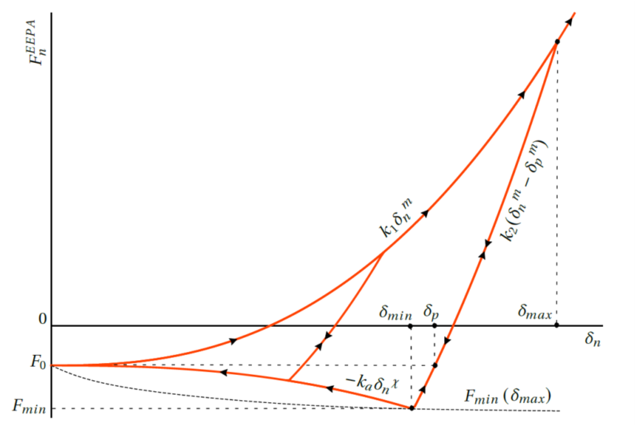
Figure 1: Force-displacement law in the normal direction.
The normal force is given by:
The contact is activated at normal overlap \(\delta_n = 0\), where the normal force jumps to a (negative) value \(F_0\). Virgin loading follows the \(k_1\)-branch defined by the stiffness \(k_1\) and the overlap \(\delta_n\) raised to the power \(m\) (the first condition in equation (2)). The maximum overlap is a history-dependent parameter and is updated and stored in the contact model.
Unloading follows the \(k_2\)-branch defined by the stiffness \(k_2\) and the plastic overlap \(\delta_p\) (the second condition in equation (2)). This branch uses the same exponent \(m\) as the \(k_1\)-branch, and the stiffness \(k_2\) is defined in terms of the plasticity ratio \(\lambda_p\), as
When \(\lambda_p=0\), then \(k_2=k_1\) and there is no plastic behavior. When \(\lambda_p \rightarrow 1\), then \(k_2 \rightarrow +\infty\) and the behavior is perfectly plastic. The stiffness \(k_1\) is defined in terms of the effective Young’s modulus \(E^*\), in a format similar to that of the classic Hertz model:
where
with \(R_1\) and \(R_2\) the radii of the two contacting pieces. If one piece is a wall facet, \(\bar{R}=R_p\), where \(R_p\) is the particle radius.
The plastic overlap is defined as the overlap where the force on the \(k_2\)-branch is equal to the pull-off force \(F_0\), and is given in terms of the maximum overlap and plasticity ratio,
Unloading along the \(k_2\)-branch results in a tensile (adhesive) force development. At the plastic overlap \(\delta_p\) the force is equal to the pull-off force \(F_0\). Further unloading follows the same branch until the magnitude of the tensile force is equal to the minimum force \(F_{min}\), which is given by:
where \(\gamma^*\) is the contact effective surface adhesion energy based on the Johnson-Kendall-Roberts (JKR) model for adhesive forces, which takes van-der-Waals effects into account([Johnson1971a]). The contact patch radius (assuming a circular contact area) \(a\) is given by Hertz’s theory, using the plastic overlap \(\delta_p\),
If the surface energy is set to zero, the adhesion branch is a horizontal line and \(F_{min} = F_0\).
Once the force is equal to \(F_{min}\) during unloading on the \(k_2\)-branch, further unloading switches to the \(k_a\)- or adhesion branch (third condition in equation (2)). The overlap exponent is \(\chi\) and the adhesion stiffness is calculated as follows, to ensure that the unloading branch results in the force being equal to \(F_{min}\) when \(\delta_n=0\):
where the overlap corresponding to the minimum force is given by:
Note that the adhesion stiffness \(k_a\) is not constant, and is indirectly dependent on the load history (dependent on \(F_{min}\), which depends on the plastic overlap \(\delta_p\), which again depends on the maximum overlap \(\delta_{max}\)).
If the contact is unloading along the \(k_2\)-branch, and then starts to reload, the same \(k_2\)-branch is followed until the \(k_1\)-branch is reached. Further virgin loading follows the \(k_1\)-branch and will result in an increased and updated \(\delta_{max}\) (and \(\delta_p\)). If the contact is unloading along the \(k_a\)-branch, and then starts to reload, a \(k_2\)-branch is followed as shown in Figure 1. In this case, the value of \(\delta_p\) is updated to the point that this \(k_2\)-branch is equal to the pull-off force \(F_0\).
On the \(k_2\)-branch, the force has a minimum limit if unloading is allowed to continue until zero overlap \(\delta_n = 0\), and, under some circumstances, it is possible the unloading branch would not reach the minimum force \(F_{min}\). The minimum force limit that can be achieved when unloading on the \(k_2\)-branch is given by:
If the minimum force given by equation (7) is less than this limit (larger in magnitude) \(F_{min} \leq F_{min}^{limit}\), the adhesion branch would never be reached and the solution for the minimum overlap \(\delta_{min}\) in equation (10) would have no real solution. This might occur when, for example, a relatively high surface energy is specified, and a specific contact has a relatively small maximum overlap. In order to avoid such a situation, the minimum force \(F_{min}\) is modified and set to the average of the pull-off force \(F_0\) and limit force \(F_{min}^{limit}\),
Shear Force \(\mathbf{F_{s}^{EEPA}}\)
In the shear direction, a trial shear force is first computed as:
where \(\left(\mathbf{F_{s}^{EEPA}}\right)_o\) is the shear force at the beginning of the timestep, \(\Delta \pmb{δ} _\mathbf{s}\) is the relative shear-displacement increment, and the tangent shear stiffness \(k_s^t\) is a function of the normal overlap \(\delta_n\) ([Morrisey2013]):
where \(G^*\) is the effective shear modulus and \(k_{sf}\) is a scaling factor.
To account for cohesive effects in the tangential direction, the Coulomb friction limit is usually modified. This is a relatively simple approach that is easy to implement and is based on the work by [Thornton1991] and [ThorntonAndYin1991], who showed that with adhesion present the contact area decreases with an increase in the tangential force. The tangential force reaches a critical value, which marks transition from a “peeling” action to a “sliding” action. Assuming the JKR theory ([Johnson1971a]), it is shown that at this critical point the contact area corresponds to a Hertzian-like normal stress distribution under a load of \((F_n^H + 2 F_{po})\), where \(F_n^H\) is the elastic force according to Hertz’s theory and \(F_{po}\) is the pull-off (maximum tensile) force ([Marshall2009]).
A similar approach is used in the EEPA model, and the updated force from equation (13) is limited by the following criteria:
where the normal force \(F_n^{EEPA}\) is given by equation (2), and the minimum force \(F_{min}\) is given by equation (12). Note that \(F_{min}\) would have a negative value, and will thus always increase the reference force \((F_n^{EEPA} - F_{min})\) which can never be smaller than zero.
If the first condition in equation (15) is met, the boolean slip state is set to \(s=\mbox{false}\), and when the second condition is met it is set to \(s=\mbox{true}\). Whenever the slip states changes, the slip_change callback event occurs.
Dashpot force
The dashpot force is resolved into normal and shear components:
In the normal direction:
where \(m_c = \frac{m_1 m_2}{m_1 + m_2}\) is the effective contact mass with \(m_1\) and \(m_2\) the mass of the two contacting particles (for a contact with a wall facet, \(m_c = m_p\) where \(m_p\) is the mass of the particle), \(\dot{\delta}_n\) is the relative normal translational velocity, \(k_n^t\) is the tangent normal stiffness, and \(\beta_n\) is the normal critical damping ratio. This ratio takes a value \(\beta_n=0\) when there is no damping, and \(\beta_n=1\) when the system is critically damped.
The tangent normal stiffness is given by:
The dashpot force in the shear direction is given by:
where \(M_d\) is the dashpot behavior mode, \(\dot{\pmb{δ}}_\mathbf{s}\) is the relative shear translational velocity, \(\beta_s\) is the shear critical damping ratio, and \(k_s^t\) is the tangential shear stiffness given by equation (14).
Rolling Resistance
The rolling resistance moment is first incremented as:
where \(k_r^t\) is the tangent rolling resistance stiffness, and \(\Delta \pmb{θ}_\mathbf{b}\) is the relative bend-rotation increment of this equation in the i Contact Resolution section.
The tangent rolling resistance stiffness \(k_r^t\) is defined as:
with \(k_s^t\) the tangent shear stiffness given by equation (14) and \(\bar{R}\) the contact effective radius (equation (5)).
The magnitude of the updated rolling resistance moment is then checked against a threshold limit:
where the same arguments used for the shear force are used to increase the limiting moment by the effects of the minimum force \(F_{min}\). The normal force \(F_n^{EEPA}\) is taken at the end of the current step, and \(\mu_r\) is the rolling coefficient of friction. If the first condition in (22) is met, then the rolling slip state is set to \(s_r=\mbox{false}\), and when the second condition is met it is set to \(s_r=\mbox{true}\).
Energy Partitions
The EEPA model provides five energy partitions:
- strain energy, \(E_{k}\), stored in the non-linear springs;
- slip energy, \(E_{\mu}\), defined as the total energy dissipated by frictional slip;
- dashpot energy, \(E_{\beta}\), defined as the total energy dissipated by the dashpots;
- rolling strain energy, \(E_{k_r}\), stored in the rolling linear spring; and
- rolling slip energy, \(E_{\mu_r}\), defined as the total energy dissipated by rolling slip.
If energy tracking is activated, these energy partitions are updated as follows:
Incrementally update the strain energy:
(23)\[\begin{split}\begin{array}{ll} E_k := E_k & + \frac{1}{2} \left(\left(F_{n}^{EEPA}\right)_o + F_{n}^{EEPA}\right) \Delta \delta_n \\ & + \frac{1}{2} \left(\left(\mathbf{F_{s}^{EEPA}}\right)_o + \mathbf{F_{s}^{EEPA}}\right) \cdot \Delta \pmb{δ}_\mathbf{s}^\mathbf{k} \\ {\rm with} & \Delta \pmb{δ} _\mathbf{s}^{k } =\Delta \pmb{δ} _\mathbf{s} -\Delta \pmb{δ} _\mathbf{s}^{\mu} = \left(\frac{\mathbf{F_{s}^{EEPA}} -\left(\mathbf{F_{s}^{EEPA}} \right)_{o} }{k_{s}^t } \right) \end{array}\end{split}\]where \(\left(F_{n}^{EEPA}\right)_o\) and \(\left(\mathbf{F_{s}^{EEPA}}\right)_o\) are, respectively, the EEPA normal and shear forces at the beginning of the step, and the relative shear-displacement increment has been decomposed into an elastic \(\left(\Delta \pmb{δ} _\mathbf{s}^{k} \right)\) and a slip \(\left(\Delta \pmb{δ} _\mathbf{s}^{\mu } \right)\) component, with \(k_s^t\) the tangent shear stiffness at the start of the current step (equation (14)).
Incrementally update the slip energy:
(24)\[E_{\mu } :=E_{\mu } - {\tfrac{1}{2}} \left(\left(\mathbf{F_{s}^{EEPA}} \right)_{o} +\mathbf{F_{s}^{EEPA}} \right)\cdot \Delta \pmb{δ} _\mathbf{s}^{\mu }\]Incrementally update the dashpot energy:
(25)\[E_{\beta } :=E_{\beta } - \mathbf{F^{d}} \cdot \left(\dot{\pmb{δ} }{\kern 1pt} {\kern 1pt} \Delta t\right)\]where \(\dot{\pmb{δ} }\) is the relative translational velocity of this equation in the i Contact Resolution section.
Update the rolling strain energy:
(26)\[E_{k_r} = \frac{1}{2} \frac{\left\| \mathbf{M^{r}} \right\| ^{2} }{k_{r}}.\]Incrementally update the rolling slip energy:
(27)\[\begin{split}\begin{array}{l} {E_{\mu_r} := E_{\mu_r} - {\tfrac{1}{2}} \biggl(\left(\mathbf{M^{r}} \right)_{o} +\mathbf{M^{r}} \biggr)\cdot \Delta \pmb{θ}_\mathbf{b}^{\mu_r} } \\ {{\rm with}\qquad \Delta \pmb{θ}_\mathbf{b}^{\mu_r} = \Delta \pmb{θ}_\mathbf{b} -\Delta \pmb{θ}_\mathbf{b}^{k} =\Delta \pmb{θ}_\mathbf{b} -\left(\frac{\mathbf{M^{r}} -\left(\mathbf{M^{r}} \right)_{o} }{k_{r}^t } \right)} \end{array}\end{split}\]where \(\left(\mathbf{M^{r}} \right)_{o}\) is the rolling resistance moment at the beginning of the timestep, and the relative bend-rotation increment has been decomposed into an elastic \(\Delta \pmb{θ}_\mathbf{b}^{k}\) and a slip \(\Delta \pmb{θ}_\mathbf{b}^{\mu_r}\) component, with \(k_{r}^t\) the tangent rolling stiffness. The dot product of the slip component and the rolling resistance moment occurring during the timestep gives the increment of rolling slip energy.
Additional information, including the keywords by which these partitions are referred to in commands and FISH, is provided in the table below.
| Keyword | Symbol | Description | Range | Accumulated |
|---|---|---|---|---|
| Hertz Group: | ||||
energy‑strain‑eepa |
\(E_{k}\) | strain energy | \((-\infty,+\infty)\) | YES |
energy‑slip |
\(E_{\mu}\) | total energy dissipated by slip | \([0.0,+\infty)\) | YES |
| Dashpot Group: | ||||
energy‑dashpot |
\(E_{\beta}\) | total energy dissipated by dashpots | \([0.0,+\infty)\) | YES |
| Rolling-Resistance Group: | ||||
energy‑rrstrain |
\(E_{k_r}\) | Rolling strain energy | \([0.0,+\infty)\) | NO |
energy‑rrslip |
\(E_{\mu_r}\) | Total energy dissipated by rolling slip | \((-\infty,0.0]\) | YES |
Properties
The properties defined by the EEPA contact model are listed in the table below for a concise reference; see the “Contact Properties” section of the “Contact Model Framework” for a description of the information in the table columns. The mapping from the surface-inheritable properties to the contact model properties is also discussed below.
| Keyword | Symbol | Description | Type | Range | Default | Modifiable | Inheritable |
|---|---|---|---|---|---|---|---|
| eepa | Model name | ||||||
| EEPA Group: | |||||||
| rgap | \(g_r\) | Reference gap [length] | FLT | \(\mathbb{R}\) | 0.0 | YES | NO |
| eepa_shear | \(G\) | Shear modulus [stress] | FLT | \((0.0,+\infty)\) | 0.0 | YES | YES |
| eepa_poiss | \(\nu\) | Poisson’s ratio [-] | FLT | \([0.0,0.5]\) | 0.0 | YES | YES |
| ks_fac | \(k_{sf}\) | Shear stiffness scaling factor [-] | FLT | \((0.0,+\infty)\) | 1.0 | YES | NO |
| fric | \(\mu\) | Sliding friction coefficient [-] | FLT | \([0.0,+\infty)\) | 0.0 | YES | YES |
| surf_adh | \(\gamma^*\) |
|
FLT | \([0.0,+\infty)\) | 0.0 | YES | NO |
| overlap_max | \(\delta_{max}\) | Maximum overlap [length] | FLT | \([0.0,+\infty)\) | 0.0 | NO | N/A |
| force_min | \(f_{min}\) | Minimum force [force] | FLT | \([0.0,+\infty)\) | 1.5 | YES | NO |
| pull_off | \(F^0\) | Pull-off force [force] | FLT | \((-\infty,0.0]\) | 0.0 | NO | NO |
| plas_ratio | \(\lambda_p\) | Plasticity ratio [-] | FLT | \((0.0,1.0)\) | 0.5 | YES | NO |
| lu_exp | \(m\) | Loading-unloading branch exponent [-] | FLT | \([1.0,+\infty)\) | 1.5 | YES | NO |
| adh_exp | \(\chi\) | Adhesive branch exponent [-] | FLT | \([1.0,+\infty)\) | 1.5 | YES | NO |
| eepa_slip | \(s\) | Slip state [-] | BOOL | {false,true} | false | NO | N/A |
| eepa_force | \(\mathbf{F^{EEPA}}\) | EEPA force (contact plane coord. system) | VEC | \(\mathbb{R}^3\) | \(\mathbf{0}\) | YES | NO |
| \(\left( -F_n^{EEPA},F_{ss}^{EEPA},F_{st}^{EEPA} \right) \quad \left(\mbox{2D model: } F_{ss}^{EEPA} \equiv 0 \right)\) | |||||||
| Rolling-Resistance Group: | |||||||
| rr_fric | \(\mu_r\) | Rolling friction coefficient [-] | FLT | \([0.0,+\infty\) | 0.0 | YES | YES |
| rr_moment | \(M^r\) | Rolling Resistance moment (contact plane coord. system) | VEC | \(\mathbb{R}^3\) | \(\mathbf{0}\) | YES | NO |
| \(\left( 0,M_{bs}^r,M_{bt}^r \right) \quad \left(\mbox{2D model: } M_{bt}^r \equiv 0 \right)\) | |||||||
| rr_slip | \(s_r\) | Rolling slip state [-] | BOOL | {false,true} | false | NO | N/A |
| Dashpot Group: | |||||||
| dp_nratio | \(\beta_n\) | Normal critical damping ratio [-] | FLT | \([0.0,1.0]\) | 0.0 | YES | NO |
| dp_sratio | \(\beta_s\) | Shear critical damping ratio [-] | FLT | \([0.0,1.0]\) | 0.0 | YES | NO |
| dp_mode | \(M_d\) | Dashpot mode [-] | INT | {0;1} | 0 | YES | NO |
| \(\;\;\;\;\;\;\begin{cases} \mbox{0: no cutt-off} \\ \mbox{1: cut-off in shear when sliding} \end{cases}\) | |||||||
| dp_force | \(\mathbf{F^{d}}\) | Dashpot force (contact plane coord. system) | VEC | \(\mathbb{R}^3\) | \(\mathbf{0}\) | NO | N/A |
| \(\left( -F_n^d,F_{ss}^d,F_{st}^d \right) \quad \left(\mbox{2D model: } F_{ss}^d \equiv 0 \right)\) | |||||||
Surface Property Inheritance
The shear modulus \(G\), Poisson’s ratio \(\nu\), friction coefficient \(\mu\) and rolling friction coefficient \(\mu_r\) may be inherited from the contacting pieces. Remember that for a property to be inherited, the inheritance flag for that property must be set to true (default), and both contacting pieces must hold a property with an identical name.
The shear modulus and Poisson’s ratio are inherited as:
with:
where (1) and (2) denote the properties of piece 1 and 2, respectively.
The friction and rolling friction coefficients are inherited using the minimum of the values set for the pieces:
Methods
No methods are defined by the EEPA model.
Callback Events
| Event | Array Slot | Value Type | Range | Description |
|---|---|---|---|---|
| contact_activated | contact becomes active | |||
| 1 | C_PNT | N/A | contact pointer | |
| slip_change | Slip state has changed | |||
| 1 | C_PNT | N/A | contact pointer | |
| 2 | INT | {0;1} | slip change mode | |
| \(\;\;\;\;\;\;\begin{cases} \mbox{0: slip has initiated} \\ \mbox{1: slip has ended} \end{cases}\) | ||||
Model Summary
An alphabetical list of the EEPA model properties is given here.
References
| [Johnson1971a] | (1, 2) Johnson, K. L., Kendall, K., and A. D. Roberts, “Surface Energy and the Contact of Elastic Solids,” Proceedings of the Royal Society of London. Series A, Mathematical and Physical Sciences, 234(1558):301-313, Sept. 1971. |
| [Marshall2009] | Marshall, J. S., “Discrete-Element Modeling of Particulate Aerosol Flows,” Journal of Computational Physics, 228(5):1541-1561, march 2009. doi:10.1016/j.jcp.2008.10.035. |
| [Morrisey2013] | (1, 2, 3) Morrissey, J. P., “Discrete Element Modelling of Iron Ore Pellets to Include the Effects of Moisture and Fines,” PhD thesis, Edinburgh, Scotland: University of Edinburgh (2013). |
| [Thornton1991] | Thornton, C., “Interparticle sliding in the presence of adhesion,” Journal of Physics D: Applied Physics, 24(11):1942-1946,1991. ISSN 13616463. doi:10.1088/0022-3727/24/11/007. |
| [ThorntonAndYin1991] | Thornton, C., and K. K. Yin, “Impact of elastic spheres with and without adhesion,” Powder Technology, 65(1-3):153-166,1991. ISSN 00325910. doi:10.1016/0032-5910(91)80178-L. |
| [WaltonBraun1986] | (1, 2) Walton, R., and R. L. Braun. “Viscosity, Granular-Temperature, and Stress Calculations for Shearing Assemblies of Inelastic, Frictional Disks,” Journal of Rheology, 30(5), pp. 949-980 (1986). |
| Was this helpful? ... | PFC © 2021, Itasca | Updated: Feb 25, 2024 |