
Solving Flow-Only and Coupled-Flow Problems
FLAC3D has the ability to perform both flow-only and coupled fluid-mechanical analyses. Coupled analysis may be performed with any of the built-in mechanical models in FLAC3D.
Several modeling strategies are available to approach the coupled processes.
One of these assumes that pore pressures once assigned to the grid do not change;
this approach does not require any extra memory to be reserved for flow calculation.
The commands associated with this mode are discussed
in Grid Not Configured for Fluid Flow.
Modeling strategies involving flow of fluid require that the model configure fluid command be issued to configure the grid for fluid analysis,
and the model configure fluid command be issued for all zones in which fluid flow can occur.
Note that for coupled analysis, the fluid-flow model is not made null automatically for zones that are made null mechanically.
The zone fluid cmodel assign null command must be given for fluid null zones.
The commands associated with model configure fluid mode are discussed
in Grid Configured for Fluid Flow.
The different modeling strategies for coupled analysis will be illustrated in the following sections, the more elaborate requiring more computer memory and time. As a general rule, the simplest possible option should be used, consistent with the reproduction of the physical processes that are important to the problem at hand. Recommended guidelines for selecting an approach based on time scales are given in Selection of a Modeling Approach for a Fully Coupled Analysis, and various modeling strategies are described in Fixed Pore Pressure to Coupled Flow and Mechanical Calculations.
Time Scales
When planning a simulation involving fluid flow or coupled flow calculations with FLAC3D, it is often useful to estimate the time scales associated with the different processes involved. Knowledge of the problem time scales and diffusivity help in the assessment of maximum grid extent, minimum zone size, timestep magnitude and general feasibility. Also, if the time scales of the different processes are very different, it may be possible to analyze the problem using a simplified (uncoupled) approach. (This approach for fully coupled analyses is discussed in detail in Selection of a Modeling Approach for a Fully Coupled Analysis.)
Time scales may be appreciated using the definitions of characteristic time given below. These definitions, derived from dimensional analysis, enter the expression of analytical continuous source solutions. They can be used to derive approximate time scales for the FLAC3D analysis.
Characteristic time of the mechanical process
where \(K_u\) is undrained bulk modulus, \(G\) is shear modulus, \(\rho\) is mass density, and \(L_c\) is characteristic length (i.e., the average dimension of the medium).
Characteristic time of the diffusion process
where \(L_c\) is the characteristic length (i.e., the average length of the flow path through the medium), and \(c\) is the diffusivity defined as mobility coefficient \(k\) divided by storativity \(S\):
There are different forms of storativity that apply in FLAC3D depending on the controlling process:
- fluid storage
- phreatic storage
- elastic storage
where \(M\) is Biot modulus, \(\alpha\) is Biot coefficient (\(M\) = \(K_f/n\) and \(\alpha\) = 1 for incompressible grains), \(K\) is drained bulk modulus, \(G\) is shear modulus, \(\rho_w\) is fluid density, \(g\) is gravity and \(L_p\) is characteristic storage length (i.e., the average height of the medium available for fluid storage).
For saturated flow-only calculations (rigid material), \(S\) is fluid storage and \(c\) is the fluid (Equation (3) and (4)):
For unsaturated flow calculations, \(S\) is phreatic storage and the diffusivity (from Equation (3) and (5)) is
For a coupled, saturated, deformation-diffusion analysis with FLAC3D, \(S\) is elastic storage and \(c\) is the true or generalized coefficient of consolidation, defined from Equation (3) and (6) as
There are some noteworthy properties based on the preceding definitions:
Because explicit timesteps in FLAC3D correspond to the shortest time needed for the information to propagate from one gridpoint to the next, the magnitude of the timestep can be estimated using the smallest zone size for \(L_c\) in the formula for characteristic time. It is important to note that the explicit fluid flow timestep in FLAC3D is calculated using the fluid diffusivity (Equation (7)), even in a coupled simulation. The timestep magnitude may thus be estimated from the formula obtained after substitution of Equation (7) in Equation (2), and using the smallest zone size \(L_z\) for \(L_c\):
(10)\[\Delta t = \min \left( {{L_z^2 } \over{k M}} \right)\]In a saturated fluid-flow problem, a reduced bulk modulus (i.e., \(M\) or \(K_f\)) leads not only to an increased timestep, but also to an increased time to reach steady state, so that the total number of steps, \(n_t\), stays the same. This number may be estimated by taking the ratio of the characteristic times for the model, \(t_c\), to the critical timestep, \(\Delta t\), using Equation (2), (7) and (10), which gives
(11)\[n_t = {\left( {L_c \over L_z} \right)}^2\]where \(L_c\) and \(L_z\) are characteristic length for the model and the smallest zone.
In a partially saturated fluid-flow problem, adjustments can be made to the fluid modulus (\(M\) or \(K_f\)) to speed convergence to steady state. Be careful not to reduce \(M\) (or \(K_f\)) so much that numerical instability results. A condition for stability may be derived from the requirement that the fluid storage (used in the critical timestep evaluation) must remain smaller than the phreatic storage over one zone height, \(L_z\):
(12)\[M > a L_z \rho_w g/n\]where \(a\) is an adjustment factor chosen equal to 0.3.
Using Equation (2), we see that, to avoid any boundary effects in diffusion problems, the characteristic length, \(L_c\), of the model must be larger than the dimension \(\sqrt{c t_s}\), where \(t_s\) is the maximum simulation time and \(c\) is the controlling diffusivity. In turn, the minimum simulation time is controlled by the relation \(t_{min} > L_z^2/c\).
In a coupled flow problem, the true diffusivity is controlled by the stiffness ratio \(R_k\) (i.e., the stiffness of the fluid versus the stiffness of the matrix):
(13)\[R_k = {{\alpha^2 M} \over {K + {4 \over 3} G}}\]With this definition for \(R_k\), Equation (14) may be expressed in two forms:
(14)\[c = k M {1 \over{1 + R_k}}\]and
(15)\[c = {k \over{\alpha^2}} \left( K + {4 \over 3} G \right) {1 \over{1 + {1 \over R_k}}}\]If \(R_k\) is small (compared to 1), Equation (9) shows that FLAC3D’s standard explicit timestep (see Equation (10)) can be considered as representative of the system diffusivity. An order-of-magnitude estimate for the number of steps needed to reach full consolidation under saturated conditions, for instance, can be calculated using Equation (11).
If \(R_k\) is large (i.e., \(M\) is large compared to \((K + 4G/3)/\alpha^2\) (or \(K_f >>> (K + 4G/3)n\))), FLAC3D’s explicit timestep will be very small, and the problem diffusivity will be controlled by the matrix (see Equation (10) and (14)). The value for \(M\) (or \(K_f\)) can be reduced in order to increase the timestep and reach steady-state computationally faster. Equation (14) indicates that if \(M\) (or \(K_f\)) is reduced such that \(R_k\) = 20, then the diffusivity should be within 5% of the diffusivity for infinite \(M\) (or \(K_f\)) (see 1D Consolidation for an example). The time scale is expected to be respected within the same accuracy. Note that, in any case, \(K_f\) should not be made higher than the physical value of the fluid (2 × 10⁹ Pa for water).
Selection of a Modeling Approach for a Fully Coupled Analysis
A fully coupled quasi-static hydromechanical analysis with FLAC3D is often time-consuming, and even sometimes unnecessary. There are numerous situations in which some level of uncoupling can be performed to simplify the analysis and speed the calculation. The following examples illustrate the implementation of FLAC3D modeling approaches corresponding to different levels of fluid/mechanical coupling. Three main factors can help in the selection of a particular approach:
- the ratio between simulation time scale and characteristic time of the diffusion process;
- the nature of the imposed perturbation (fluid or mechanical) to the coupled process; and
- the ratio of the fluid to solid stiffness.
The expressions for characteristic time, \(t_c^{f}\) (in Equation (2)), diffusivity, \(c\) (in Equation (9)), and the stiffness ratio, \(R_k\) (in Equation (13)) can be used to quantify these factors. These factors are considered in detail below, and a recommended procedure to select a modeling approach based on these factors is given in Recommended Procedure to Select a Modeling Approach.
Time Scale
We first consider the time scale factor by measuring time from the initiation of a perturbation. We define \(t_s\) as the required time scale of the analysis, and \(t_c\) as the characteristic time of the coupled diffusion process (estimate of time to reach steady state, defined using Equation (2) and Equation (9)).
Short-term behavior
If \(t_s\) is very short compared to the characteristic time, \(t_c\), of the coupled diffusion process, the influence of fluid flow on the simulation results will probably be negligible, and an undrained simulation can be performed with FLAC3D (using either a “dry” or “wet” simulation — see No Flow. The wet simulation is carried out usingmodel configure fluidandzone fluid activeoff). No real time will be involved in the numerical simulation (i.e., \(t_s <<< t_c\)), but the pore pressure will change due to volumetric straining if the fluid modulus (\(M\) or \(K_f\)) is given a realistic value. The footing load simulation is an example of this approach.
Long-term behavior
If \(t_s >>> t_c\), and drained behavior prevails at \(t = t_s\), then the pore-pressure field can be uncoupled from the mechanical field. The steady-state pore-pressure field can be determined using a fluid-only simulation (zone fluid activeon,zone mechanical activeoff) (the diffusivity will not be representative), and the mechanical field can be determined next by cycling the model to equilibrium in mechanical mode with \(K_f\) = 0 (zone mechanical activeon,zone fluid activeoff). (Strictly speaking, this engineering approach is only valid for an elastic material, because a plastic material is path-dependent.)
Another way to describe the time scale is in terms of undrained or drained response. Undrained strictly means that there is no exchange of fluid with the outside world (where outside world means outside the sample in a lab test, and other elements in a numerical simulation or a field situation). Drained means that there is a full exchange of fluid with the outside world, which implies that the fluid pressure is able to dissipate everywhere. The words are typically associated with short-term and long-term, respectively, because an undrained test usually can be done quickly, while a drained test requires a long time for excess fluid pressures to dissipate. In the field, short-term means that there is insignificant migration of fluid, and long-term means that the pressure has stabilized (which needs a long time).
Note that in simulations conducted outside of the fluid configuration, or within the fluid configuration but with fluid turned off, the total stress adjustments due to an imposed pore-pressure change (such as those resulting from the lowering of the water table) will not be done internally by the code. The pore-pressure increments may, however, be monitored (using a FISH function, for instance) and used to decrement the total normal stresses before cycling to mechanical equilibrium. The saturated and unsaturated mass densities will also need to be adjusted if the water table has been moved within the grid, and the simulation is conducted outside of the fluid configuration. (See Verification of Concepts, and Modeling Techniques for Specific Applications for additional information on this topic.)
Nature of Imposed Perturbation to the Coupled Process
The imposed perturbation to a fully coupled hydromechanical system can be due to changes in either the fluid flow boundary condition or the mechanical boundary condition. For example, transient fluid flow to a well located within a confined aquifer is driven by the change in pore pressures at the well. The consolidation of a saturated foundation as a result of the construction of a highway embankment is controlled by the mechanical load applied by the weight of the embankment. If the perturbation is due to change in pore pressures, it is likely that the fluid flow process can be uncoupled from the mechanical process. This is described in more detail below, and illustrated in Transient Fluid Flow to a Well in a Shallow Confined Aquifer. If the perturbation is mechanically driven, the level of uncoupling depends on the fluid versus solid stiffness ratio, as described below.
Stiffness Ratio
The relative stiffness, \(R_k\) (see Equation (13)), has an important influence on the modeling approach used to solve a hydromechanical problem:
Relatively stiff matrix (\(R_k <<< 1\))
If the matrix is very stiff (or the fluid highly compressible) and \(R_k\) is very small, the diffusion equation for the pore pressure can be uncoupled, since the diffusivity is controlled by the fluid (Detournay and Cheng 1993). The modeling technique will depend on the driving mechanism (fluid or mechanical perturbation):
- In mechanically driven simulations, the pore pressure may be assumed to remain constant. In an elastic simulation, the solid behaves as if there were no fluid; in a plastic analysis, the presence of the pore pressure may affect failure. This modeling approach is adopted in slope stability analyses (see Fixed Pore Pressure).
- In pore pressure-driven elastic simulations (e.g., settlement caused by fluid extraction), volumetric strains will not significantly affect the pore-pressure field, and the flow calculation can be performed independently (
zone fluid activeon,zone mechanical activeoff). (In this case, the diffusivity will be accurate because for \(R_k <<< 1\), the generalized consolidation coefficient in Equation (9) is comparable to the fluid diffusivity in Equation (7).) In general, the pore-pressure changes will affect the strains, and this effect can be studied by subsequently cycling the model to equilibrium in mechanical mode (zone mechanical activeon,zone fluid activeoff). The fluid modulus (\(M\) or \(K_f\)) must be set to zero during mechanical cycling, to prevent additional generation of pore pressure.
Relatively soft matrix (\(R_k >>> 1\))
If the matrix is very soft (or the fluid incompressible) and \(R_k\) is very large, then the system is coupled, with a diffusivity governed by the matrix. The modeling approach will also depend on the driving mechanism.
- In mechanically driven simulations, calculations can be time-consuming. As discussed in note 5 of Time Scale, it may be possible to reduce the value for \(M\) (or \(K_f\)), such that \(R_k\) = 20, and not significantly affect the response.
- In most practical cases of pore pressure-driven systems, experience shows that the coupling between pore pressure and mechanical fields is weak. If the medium is elastic, the numerical simulation can be performed with the flow calculation in flow-only mode (
zone fluid activeon,zone mechanical activeoff) and then in mechanical-only mode (zone mechanical activeon,zone fluid activeoff with fluid modulus set to zero) to bring the model to equilibrium.It is important to note that, in order to preserve the true diffusivity (and hence the characteristic time scale) of the system, the fluid modulus \(M\) (or \(K_f\)) must be adjusted to the value
or
during the flow calculation (see Equation (9)), and to zero during the mechanical calculation to prevent further adjustments by volumetric strains (Berchenko 1998).
Recommended Procedure to Select a Modeling Approach
It is recommended that the selection of a modeling approach for a fully coupled analysis follow the procedure outlined in Table 1. First, determine the characteristic time of the diffusion process for the specific problem conditions and properties (see Time Scale), and compare this time to the actual time scale of interest. Second, consider whether the perturbation to the system is primarily pore-pressure driven or mechanically driven. Third, determine the ratio of the stiffness of the fluid to the stiffness of the solid matrix. Table 1 indicates the appropriate modeling approach based on the evaluation of these three factors. The table also indicates the required adjustment to the fluid modulus, \(M_a\) (or \(K_f^a\)), for each case. Finally, the table lists several examples from the manual that illustrate each modeling approach.
| Time Scale | Imposed Process Perturbation | Fluid vs Solid Stiffness | Modeling Approach & Main Calculation Commands | Adjust Fluid Bulk Modulus (\(M^a\) or \(K_f^a\)) | Examples (6) |
|---|---|---|---|---|---|
| \(t_s >>> t_c\) | mechanical or pore pressure | any \(R_k\) | Effective Stress (1) | no fluid | Curvature Slope Stability |
| (steady-state analysis) | with no fluid flow | ||||
| or | |||||
| Effective Stress (2) | \(M^a\) = 0.0 (or \(K_f^a\) = 0.0) | ||||
model configure fluid |
|||||
zone fluid active off |
|||||
zone mechanical active on |
|||||
| \(t_s <<< t_c\) | mechanical or pore pressure | any \(R_k\) | Pore Pressure Generation (3) | realistic value for \(M^a\) (or \(K_f^a\)) | Footing on Saturated Soil - Adding Load |
| (undrained analysis) | model configure fluid |
Triaxial Compression Test on a Cam-Clay Sample | |||
zone fluid active off |
|||||
zone mechanical active on |
|||||
| \(t_s\) in the range of \(t_c\) | pore pressure | any \(R_k\) | Uncoupled Flow-Mechanical (4) | 1D Consolidation - Uncoupled | |
model configure fluid |
|||||
| step 1 | \(M^a = {{1} \over {{1 \over M} + {\alpha^2 \over {K+ 4 G/3}} }}\) | ||||
zone fluid active on |
(or \(K_f^a = {{n} \over {{n \over K_f} + {1 \over {K+ 4 G/3}} }}\)) | ||||
zone mechanical active off |
|||||
| step 2 | \(M^a\) = 0.0 (or \(K_f^a\) = 0.0) | ||||
zone fluid active off |
|||||
zone mechanical active on |
|||||
| \(t_s\) in the range of \(t_c\) | mechanical | any \(R_k\) | Coupled Flow-Mechanical (5) | realistic value for \(M^a\) (or \(K_f^a\)) | Footing on Saturated Soil - Coupled |
model configure fluid |
so that \(R_k \le 20\) | 1D Consolidation - Coupled | |||
zone fluid active on |
Consolidation Settlement | ||||
zone mechanical active on |
Pressuremeter Test |
Notes to Table 1:
The effective stress approach with no fluid flow is discussed in Fixed Pore Pressure. In order to establish the initial conditions for this effective stress analysis, use the
zone water planecommand, thezone gridpoint initialize pore-pressurecommand or a FISH function to establish steady-state pore pressures. Specify the correct wet density to zones below the water table, and dry density to zones above.The effective stress approach with groundwater flow is discussed in Flow-Only Calculation. In order to establish the initial conditions for this effective stress analysis, use the
zone gridpoint initialize pore-pressurecommand or a FISH function to establish steady-state pore pressures, or specifyzone fluid activeon andzone mechanical activeoff and step to steady state if the location of the phreatic surface is not known. Set \(M^a\) (or \(K_f^a\)) to a small value to speed convergence for a partially saturated system. Note that \(M^a\) (or \(K_f^a\)) should be greater than \(0.3nL_{z}\rho_{w}g\) (or \(0.3L_{z}\rho_{w}g\)) to satisfy numerical stability (see Equation (12)).The pore-pressure generation approach is discussed in No Flow — Mechanical Generation of Pore Pressure. In order to establish the initial conditions for the pore-pressure generation analysis, use the
zone gridpoint initialize pore-pressurecommand or a FISH function to establish steady-state flow, or specifyzone fluid activeoff andzone mechanical activeon and step to steady state if the location of the phreatic surface is not known. Set \(M^a\) (or \(K_f^a\)) to a small value to speed convergence for a partially saturated system. Note that \(M^a\) (or \(K_f^a\)) should be greater than \(0.3nL_{z}\rho_{w}g\) (or \(0.3L_{z}\rho_{w}g\)) to satisfy numerical stability (see Equation (12)).The uncoupled fluid-mechanical approach is described in Selection of a Modeling Approach for a Fully Coupled Analysis. This approach is recommended for pore pressure-driven systems, and should be used carefully if \(R_k >>> 1\). Note that the adjusted value for \(M^a\) (or \(K_f^a\)) during the flow-only step should satisfy Equation (16) so that the coupled diffusivity will be correct.
The fully coupled approach is discussed in Coupled Flow and Mechanical Calculations. Note that for \(R_k >>> 1\), if \(M^a\) (or \(K_f^a\)) is adjusted to reduce \(R_k\) = 20, the time response will be close (typically within 5%) to that for infinite \(M\) (or \(K_f\)).
The saturated fast-flow option for fully coupled analysis (
zone fluid fastflowon) is discussed in Fully Saturated Fast Flow. Note that this method can only be applied for fully saturated flow. ther limitations are discussed in Fully Saturated Fast Flow.Examples are given in Verification Examples on Fluid. Example Applications (E.A.) and Verification Problems (V.P.) that demonstrate the various methods are in the Example Problems and Verification Problems.
Fixed Pore Pressure (Used in Effective Stress Calculation)
In some calculations, the pore-pressure distribution is important only because it is used in the computation of effective stress at all points in the system. For example, in modeling slope stability, we may be given a fixed water table. To represent this system with FLAC3D, it is sufficient to specify a pore-pressure distribution that is unaffected by mechanical deformations that may occur. Because no change in pore pressures is involved, we do not need to configure the grid for groundwater flow.
The zone water set command can be used to specify an initial hydrostatic pore-pressure distribution below a given fixed phreatic surface.
The water density must be provided (with the zone water density command),
and appropriate dry and saturated material densities supplied by the user above and below the water table, respectively.
Alternatively, the zone gridpoint initialize pore-pressure command or a FISH function can be used
to generate the required static pore-pressure distribution.
The pore-pressure distribution corresponds to an initial state for which there is no strain. It remains constant and is unaffected by mechanical deformation. Fluid flow does not take place. The influence of this pore-pressure distribution is on failure in material for which yield depends on mean effective stress. For an example application, see Curvature Slope Stability.
Flow-Only Calculation to Establish a Pore-Pressure Distribution
Flow-only calculations may be performed to determine the flow and pressure distribution in some system independent of any mechanical effects. For example, it may be necessary to evaluate the groundwater changes that result from the digging of a drainage ditch or the activation of a pumping well. In other instances, an initial pore-pressure distribution may be needed for a coupled calculation. In both cases, FLAC3D may be run in the fluid-flow mode without any mechanical calculation being done. Mechanical calculations may or may not be done subsequently.
The first step in the command procedure for a flow-only calculation is to issue a model configure fluid command
so that extra memory can be assigned for the fluid-flow calculation.
The mechanical calculation should be inhibited with the zone mechanical active off command.
Then a choice must be made between the explicit and implicit fluid-flow solution algorithm.
By default, the explicit algorithm will be selected,
but the implicit mode of calculation may be activated (and deactivated) at any stage of the calculation
using the zone fluid implicit on or zone fluid implicit off command.
Note however, that the implicit calculation mode only applies to problems
in which the medium remains fully saturated (i.e., the saturation remains constant and equal to one);
it will give wrong results if desaturation occurs in the simulation.
When using the implicit mode of calculation, always make sure that desaturation has not taken place
(e.g., by plotting saturation contours).
In the explicit mode, the fluid-flow timestep will be calculated automatically,
but a smaller timestep can be selected using the model fluid timestep command.
The magnitude of the timestep must be specified by the user in the implicit mode.
This is done by issuing a model fluid timestep command.
For saturated flow, it is often more efficient to use the implicit solution mode when contrasting permeabilities exist.
The fluid-flow model and properties must be specified for all zones in which fluid flow may occur.
Initial and boundary conditions are assigned to complete the fluid-flow problem setup.
The fluid-flow domain in a fluid-only or fluid-mechanical simulation is defined by the assembly of zones with a non-null fluid flow model.
Flux boundary conditions, for instance, can be assigned by specifying the zone face apply flux command
with the range keyword to correspond to the boundaries of that domain.
(Remember that zones that are nulled mechanically are not automatically nulled for fluid flow.)
The model step command may be specified to execute a given number of fluid-flow steps.
To stop the calculation automatically when a particular fluid-flow time is reached,
a model solve command may be issued.
Alternatively, the model solve fluid time-total or model solve fluid cycles setting
may be specified to prescribe a fluid-flow time limit or maximum number of steps;
then a model solve command may be given.
A steady-state flow condition can also be calculated by using the model solve command
with the ratio keyword to specify the limiting unbalanced fluid-flow ratio defining the steady flow state.
If the computed pore-pressure distribution is then to be used in a mechanical calculation
where pore pressure can be assumed to remain constant,
the zone fluid active off and zone mechanical active on commands should be given.
The Biot coefficient or fluid bulk modulus should also be set to zero
to prevent extra pore pressures from being generated by mechanical deformation.
Steady-State Fluid Flow with a Free Surface presents an example flow-only analysis in which unconfined flow through a vertical embankment is calculated. The analysis produces the steady-state phreatic surface. Note that in this example, the fluid bulk modulus is set to a low value to enable the phreatic surface to develop quickly. This can be done when the time taken to reach steady state is unimportant. Note, however, that there is a lower limit for fluid modulus in order to avoid numerical instability (see Equation (12)).
No Flow — Mechanical Generation of Pore Pressure
The undrained (short-term) response may be analyzed in FLAC3D using both dry and wet approaches.
In a dry simulation, the generation of pore pressure under volumetric strain is not simulated directly.
Instead, its effect on mechanical deformation is taken into account by assigning the undrained bulk value,
\(K_u = K + \alpha^2 M\), to the material bulk modulus, \(K\), in the FLAC3D simulation.
In this case, two different techniques can be applied to detect failure in a Mohr-Coulomb material.
In the first one, the constant pore pressures are initialized using the zone water or zone gridpoint initialize pore-pressure command,
and undrained cohesion and friction are given as input.
In the second, the material is assigned a zero friction and a cohesion equal to the undrained shear strength, \(C_u\).
The first technique applies to problems where changes in pore pressure are small compared to the initial values.
The second technique strictly applies to plane-strain problems with Skempton coefficient equal to one (\(M >>> K + 4G/3\)).
Note that a dry simulation can be carried out whether or not the model configure fluid command has been issued.
However, if the command has been used, the fluid bulk modulus (\(M\) or \(K_f\)) must be set to zero to prevent additional generation of pore pressure.
In a wet simulation, the short-term response of a coupled system is analyzed in the fluid configuration of FLAC3D.
In this case, drained values should be used for the material bulk modulus, friction and cohesion.
If the zone fluid active off command is given, and the Biot modulus (or fluid modulus) is given a realistic value,
then pore pressure will be generated as a result of mechanical deformations.
For example, the “instantaneous” pore pressures produced by a footing load can be computed in this way.
If the fluid bulk modulus (\(M\) or \(K_f\)) is much greater than the solid bulk modulus, convergence will be slow;
it may be possible to reduce the fluid bulk modulus without significantly affecting the behavior.
(See Note 5 in Table 1.)
The data file Footing-InstantPP.dat illustrates pore pressure buildup produced by a footing load on an elastic/plastic material contained in a box.
The corresponding project file, “Footing.prj,’’ is located in the “datafiles\Fluid\Footing” folder.
The left boundary of the box is a line of symmetry, and the pore pressure is fixed at zero along the top surface to prevent pore-pressure generation there.
By default, the porosity is 0.5; permeability is not needed, since flow is not calculated.
Note that the pore pressures are fixed at zero at gridpoints along the top of the grid.
This is done because at the next stage of this model, a coupled,
drained analysis in which drainage will be allowed at the ground surface will be performed
(see Coupled Flow and Mechanical Calculations).
The zero pore-pressure condition is set now to provide the compatible pore-pressure distribution for the second stage.
As a large amount of plastic flow occurs during loading,
the normal stress is applied gradually by using the FISH function ramp
to supply a linearly varying multiplier to the zone apply command.
Figure 1 shows pore-pressure contours and vectors representing the applied forces.
It is important to realize that the plastic flow will occur in reality over a very short period of time (on the order of seconds);
the word “flow” here is misleading since, compared to fluid flow, it occurs instantaneously.
Hence, the undrained analysis (with zone fluid active off) is realistic.
The saturated fast-flow logic can be used for this example because the material is fully saturated,
and the stiffness of the fluid is significantly greater than that of the solid matrix.
It is only necessary to include the zone fluid fastflow on command
in Footing-InstantPP.dat
to perform a saturated fast-flow calculation.
Calculational stepping stops, and equilibrium is achieved,
when the unbalanced volumes, \(V_{av}\) and \(V_{max}\),
and the unbalanced force ratio are smaller than the predefined limits.
The instantaneous pore-pressure generation is nearly the same (within approximately 5%) as that obtained by the basic flow scheme,
as illustrated in Figure 2.
The runtime for the saturated fast-flow scheme is roughly three times faster than that for the basic flow scheme.
Footing-InstantPP.dat:
model new
model large-strain off
model title 'Instantaneous pore pressures generated under an applied load'
model configure fluid
zone create brick size 40 1 20 point 0 (0,0,0) point 1 (20,0, 0) ...
                               point 2 (0,1,0) point 3 ( 0,0,10)
; --- mechanical model ---
zone cmodel assign mohr-coulomb
zone property bulk 5e7 shear 3e7 fric 25 cohesion 1e5 tens 1e10
zone gridpoint fix velocity-x  range union position-x 0 position-x 20
zone gridpoint fix velocity-y
zone gridpoint fix velocity-z  range position-z 0
; --- apply load slowly ---
fish define ramp
    ramp = math.min(1,global.step/1000)
end
zone face apply stress-normal = -0.3e6 fish ramp ...
                range position-x 0 3 position-z 10
; --- fluid flow model ---
zone fluid cmodel assign isotropic
zone gridpoint initialize fluid-modulus 9e8
; --- pore pressure fixed at zero at the surface ---
zone gridpoint fix pore-pressure 0 range position-z 10
; --- settings ---
model fluid active off
; --- histories ---
zone history pore-pressure position (2,1,9)
; --- timing ---
[global t0 = time.clock/100]
model solve convergence 1
[(time.clock/100)-t0]
model save 'load'
program return
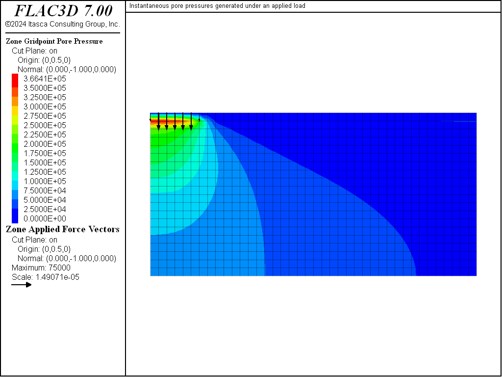
Figure 1: Instantaneous pore pressures generated under an applied load.
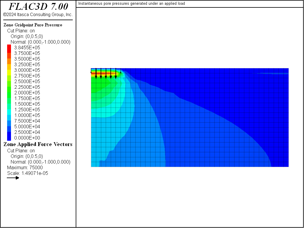
Figure 2: Instantaneous pore pressures generated under an applied load — with zone fluid fastflow on.
Coupled Flow and Mechanical Calculations
By default, FLAC3D will do a coupled fluid-flow and mechanical calculation if the grid is configured for fluid, and if the Biot modulus, or fluid bulk modulus, and permeability are set to realistic values. The full fluid-mechanical coupling in FLAC3D occurs in two directions: pore-pressure changes cause volumetric strains that influence the stresses; in turn, the pore pressure is affected by the straining that takes place.
The relative time scales associated with consolidation and mechanical loading should be appreciated. Mechanical effects occur almost instantaneously (on the order of seconds, or fractions of seconds). However, fluid flow is a long process: the dissipation associated with consolidation takes place over hours, days or weeks.
Relative time scales may be estimated by considering the ratios of characteristic times for the coupled and undrained processes. The characteristic time associated with the undrained mechanical process is found by using the saturated mass density for \(\rho\) and the undrained bulk modulus, \(K_u\), as defined in this equation (or this equation for incompressible grains) for \(K\) in Equation (1). The ratio of the diffusion characteristic time (Equation (2) and (9)) and the undrained mechanical characteristic time is thus
In most cases, \(M\) is approximately 1010 Pa, but the mobility coefficient \(k\) may differ by several orders of magnitude; typical values are
10-19m2/Pa-sec for granite;
10-17m2/Pa-sec for limestone;
10-15m2/Pa-sec for sandstone;
10-13m2/Pa-sec for clay; and
10-7m2/Pa-sec for sand.
For rock and soil, \(\rho\) is of the order of 103kg/m3, while \(K + 4/3 G\) is approximately 1010 Pa. Using those orders of magnitude in Equation (18), we see that the ratio of fluid-to-mechanical time scales may vary between \(L_c\) for sand, 106\(L_c\) for clay, 108\(L_c\) for sandstone, 1010 \(L_c\) for limestone and 1012 \(L_c\) for granite. If we exclude materials with mobility coefficients larger than that of clay, we see that this ratio remains very large, even for small values of \(L_c\).
In practice, mechanical effects can then be assumed to occur instantaneously when compared to diffusion effects. This is also the approach adopted in FLAC3D, where no time is associated with any of the mechanical steps taken together with the fluid-flow steps. The use of the dynamic option in FLAC3D may be considered, to study the fluid-mechanical interaction in materials such as sand, where mechanical and fluid time scales are comparable.
In most modeling situations, the initial mechanical conditions correspond to a state of equilibrium that must first be achieved before the coupled analysis is started.
Typically, at small fluid-flow time (compared to \(t_c\) — see Time Scale),
a certain number of mechanical steps must be taken for each fluid step to reach quasi-static equilibrium. At larger fluid-flow time,
if the system approaches steady-state flow,
several fluid-flow timesteps may be taken without significantly disturbing the mechanical state of the medium.
A corresponding numerical simulation may be controlled manually by alternating
between flow-only (zone fluid active on and zone mechanical active off)
and mechanical-only (zone fluid active off and zone mechanical active on) modes.
The model step command can be used to perform calculations for both the flow-only and mechanical-only processes.
As an alternative approach,
the tedious task of switching between flow-only and mechanical-only modes may be avoided
by using the model solve command in combination with appropriate settings;
model solve mechanical unbalanced-maximum (or model solve mechanical ratio-maximum) will set a limit to the maximum out-of-balance force (or force ratio),
under which quasi-static mechanical equilibrium will be assumed.
model mechanical substep n auto declares the mechanical module as the slave that must perform n sub-cycles
(or fewer, if equilibrium is detected — see previous setting) for each step taken by the master.
model fluid substep m implicitly declares the flow module as the master.
(The keyword auto is omitted for the master process.)
If for each fluid-flow timestep the mechanical module needs only one sub-step to reach equilibrium,
then the number of fluid-flow sub-steps is doubled, but never exceeds the number m (by default, m = 1).
The system reverts to the original setting of sub-steps whenever the succession of one mechanical timestep for each fluid-flow group of sub-steps is broken.
If the option time-total is specified in the model solve fluid command,
the computation will proceed until the fluid-flow time given by the model solve time-total parameter is reached.
In a third approach, the model step command may be used while both mechanical and fluid-flow modules are on.
In this option, one mechanical step will be taken for each fluid-flow step.
Here, fluid-flow steps are assumed to be so small that one mechanical step is enough.
Input Instructions should be consulted for a complete list of available command options for a coupled analysis.
To illustrate a fully coupled analysis,
we continue the footing simulation
(done in No Flow — Mechanical Generation of Pore Pressure),
using the model solve command with appropriate settings to calculate the consolidation beneath the footing.
The data file is Footing-Coupled.dat:
Footing-Coupled.dat:
model restore 'load'
; --- turn on fluid flow model ---
zone fluid property permeability 1e-12
model fluid active on
zone gridpoint initialize velocity (0,0,0)
zone gridpoint initialize displacement (0,0,0)
; --- set mechanical limits ---
model mechanical substep 100
model mechanical slave on
model fluid substep 10
; --- histories ---
model history fluid time-total
zone history displacement-z position 0,1,10
zone history displacement-z position 1,1,10
zone history displacement-z position 2,1,10
zone history pore-pressure  position 2,1,9
zone history pore-pressure  position 5,1,5
zone history pore-pressure  position 10,1,7
zone gridpoint initialize ratio-target 1e-3 range position-x 4 21
; --- solve to 3,000,000 sec ---
[global t0 = time.clock/100]
model solve fluid time-total 3.0e6 or mechanical convergence 10
[(time.clock/100)-t0]
model save 'age_3e6'
program return
The screen printout should be watched during the calculation process
– eight variables are updated on the screen after the model solve command is issued:
- the current step number;
- the total number of sub-cycles taken by the master process (fluid flow) for the most recent step;
- the total number of sub-cycles taken by the slave process (mechanical) for the most recent step;
- the process that is currently active;
- the current sub-cycle number;
- the current maximum unbalanced force or force ratio;
- the total time for the master (fluid flow) process; and
- the current timestep.
The unbalanced force ratio tolerance is 10-4 for this problem;
enough mechanical steps are taken to keep the unbalanced force ratio below this tolerance.
However, the limit to mechanical steps, defined by model mechanical substep, is set to 100 in this example.
If the actual number of mechanical steps taken is always equal to the set value of model mechanical substep,
then something must be wrong.
Either the force limit or model mechanical substep has been set too low, or the system is unstable and cannot reach equilibrium.
The quality of the solution depends on the force tolerance:
a small tolerance will give a smooth, accurate response,
but the run will be slow;
a large tolerance will give a quick answer, but it will be noisy.
The characteristic diffusion time for this coupled analysis is evaluated from Equation (2), using Equation (9) for the diffusivity and a value of \(L_c\) = 10 m corresponding to the model height. Using the property values in this example, \(t_c^{f}\) is estimated at 1,200,000 seconds. Full consolidation is expected to be reached within this time scale; the numerical simulation is carried out for a total of 3,000,000 seconds.
Figure 3 shows the time histories to 3,000,000 seconds of displacements under the footing load. In this simulation, pore pressures remain fixed at zero on the ground surface; hence, the excess fluid escapes upward. The leveling off of the histories indicates that full consolidation has been reached.
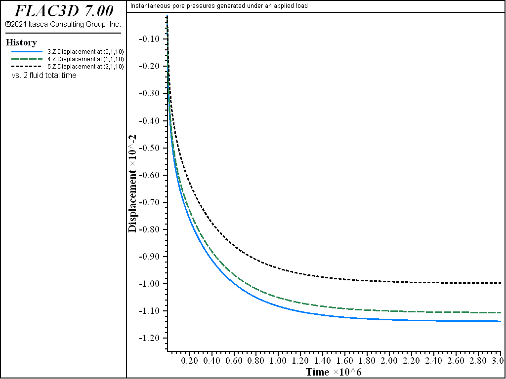
Figure 3: Consolidation response — time histories of footing displacements.
The coupled simulation can also be run using the saturated fast-flow scheme because the foundation material is fully saturated.
In this case the zone fluid fastflow on command is invoked.
When the fluid flow is turned on, the coupled calculation will continue using the saturated fast-flow scheme.
The results are similar to the results for the basic flow case, as indicated
by Figure 4 (compare to Figure 3).
The unbalanced force ratio tolerance is set to 10-6 for this simulation, in order to provide a smoother displacement history.
Even with this lower tolerance, the saturated fast-flow run is approximately 10 times faster than the basic flow simulation.
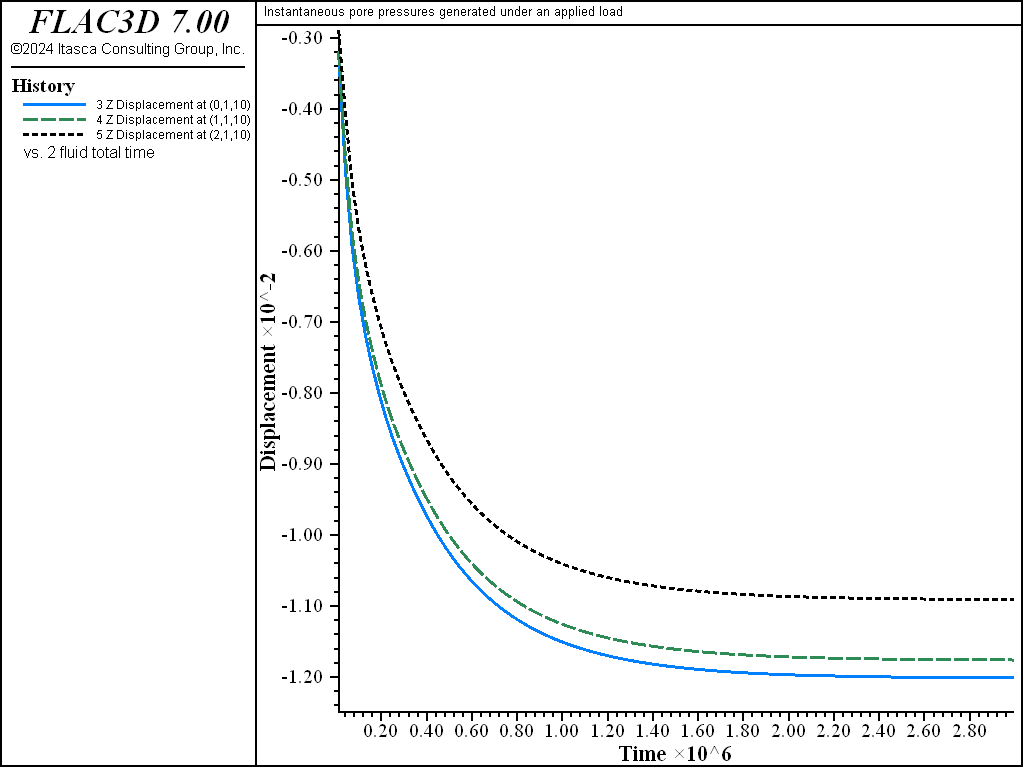
Figure 4: Consolidation response — time histories of footing displacements — with zone fluid fastflow on.
Finally, a comparison is made with an uncoupled drained analysis. First, a flow only calculation is made, then a mechanical only calculation is performed, with fluid bulk modulus set to zero. The data file for the uncoupled run is Footing-Uncoupled.dat. The displacement histories for the uncoupled drained simulation are plotted in Figure 5. The final settlement match within 3% of the basic flow results.
Footing-Uncoupled.dat:
model restore 'load'
; --- turn on fluid flow model ---
zone fluid property permeability 1e-12
model fluid active on
zone gridpoint initialize velocity (0,0,0)
zone gridpoint initialize displacement (0,0,0)
; --- histories ---
model history fluid time-total
zone history displacement-z position 0,1,10
zone history displacement-z position 1,1,10
zone history displacement-z position 2,1,10
zone history pore-pressure  position 2,1,9
zone history pore-pressure  position 5,1,5
zone history pore-pressure  position 10,1,7
; --- solve to 2,000,000 sec ---
; --- uncoupled ---
model fluid active on
model mechanical active off
model solve fluid time-total 3.0e6
model fluid active off
model mechanical active on
zone gridpoint initialize fluid-modulus 0
model solve convergence 1
model save 'age_3e6_uncoup'
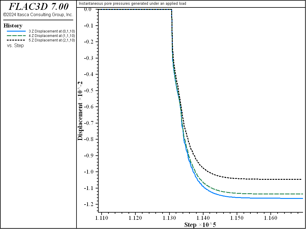
Figure 5: Consolidation response — footing displacements for uncoupled drained analysis.
If a sudden change of loading or mechanical boundary condition is applied in a coupled problem,
it is important to allow the undrained (short-term) response to develop before allowing flow to take place.
In other words, FLAC3D should be run to equilibrium under zone fluid active off conditions following the imposed mechanical change.
The model solve logic can then be used (with zone fluid active on) to compute the subsequent coupled flow/mechanical response.
If changes in fluid boundary conditions occur physically at the same time as mechanical changes,
then the same sequence should be followed
(i.e., mechanical changes | equilibrium | fluid changes | coupled solution).
Another example of fully coupled behavior is the time-dependent swelling that takes place following the excavation of a trench in saturated soil.
In this case, negative pore pressures build up immediately after the trench is excavated;
the subsequent swelling is caused by the gradual influx of water into the region of negative pressures.
We model the system in two stages:
in the first, we allow mechanical equilibrium to occur, without flow; then we allow flow,
using the model solve command to maintain quasi-static equilibrium during the consolidation process.
The fluid tension is initialized to a large negative number to prevent desaturation.
The data file used is Swelling.dat.
The corresponding project file is “Swelling.prj,” located in the “datafiles\Fluid\Swelling” folder.
The trench is excavated in the left-hand part of a flat soil deposit that is initially fully saturated and in equilibrium under gravity. The material is elastic in this case, but it could equally well have been a cohesive material, such as clay. In this run, we assume impermeable conditions for the free surfaces. Figure 6 shows the displacement vectors that accumulate during the time that flow is occurring; the trench is seen at the left-hand side of the model. Figure 7 shows the time history of pore pressure near the crest of the trench; note that there is an initial negative excursion in pressure arising from the instantaneous expansion of the soil toward the trench. Figure 8 shows histories of horizontal and vertical displacement at the crest. The characteristic time for this problem, evaluated using the model length of 40 m for \(L_c\), is approximately 5 × 10⁸ seconds (based on Equation (2) and (9)); the numerical simulation is carried out to that time.
Swelling.dat:
model new
model large-strain off
model title "Maintaining equilibrium under time-dependent swelling conditions"
model config fluid
zone create brick size 40 1 8
; --- mechanical model ---
zone cmodel assign elastic
zone property bulk 2e8 shear 1e8
zone initialize density 1500
zone cmodel assign null range position-x 0,2 position-z 2,8
; --- fluid flow model ---
zone fluid cmodel assign isotropic
zone fluid property permeability 1e-14  poros 0.5
zone gridpoint initialize fluid-modulus 2e9
zone gridpoint initialize fluid-tension -5e5
zone initialize fluid-density 1000
zone fluid cmodel assign null range position-x 0,2 position-z 2,8
; initial and boundary conditions
zone gridpoint fix velocity-x  range position-x 0
zone gridpoint fix velocity-x  range position-x 40
zone gridpoint fix velocity    range position-z 0
zone gridpoint fix velocity-y
model gravity 0,0,-10
zone initialize stress-xx -1.6e5 grad 0,0,20000
zone initialize stress-yy -1.6e5 grad 0,0,20000
zone initialize stress-zz -1.6e5 grad 0,0,20000
zone gridpoint initialize pore-pressure 8.0e4 grad 0,0,-10000
; --- settings ---
model fluid active off
;
model history mechanical unbalanced-maximum
model solve
model save 'swell1'
;
zone gridpoint initialize displacement (0,0,0)
history interval 100
model history fluid time-total
;fish history [] gp pp 3,0,7
zone history pore-pressure position 4.5,0.5,6.5
zone history displacement-x position 2,0,8
zone history displacement-z position 2,0,8
zone gridpoint fix pore-pressure range position-x 40
model fluid active on
model fluid substep 100
model mechanical substep 100
model mechanical slave   on
model solve fluid time-total 5e8 or mechanical unbalanced-maximum 50
model save 'swell2'
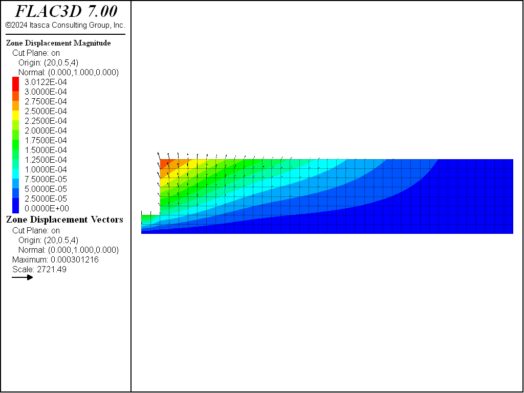
Figure 6: Swelling displacements near a trench with impermeable surfaces.
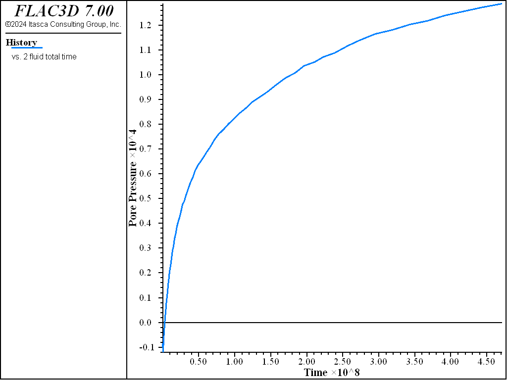
Figure 7: History of pore pressure behind the trench face.
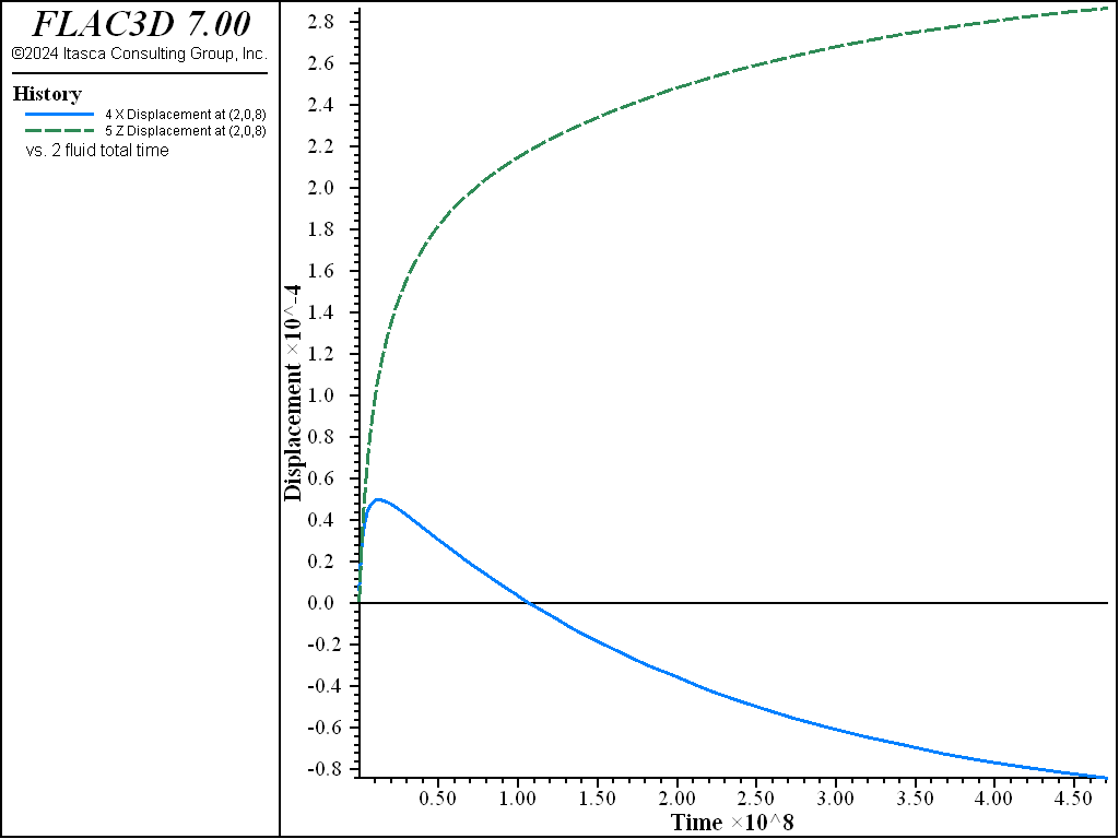
Figure 8: Displacement histories at the trench crest — vertical (top) and horizontal (bottom)
| Was this helpful? ... | PFC © 2021, Itasca | Updated: Feb 25, 2024 |