
Installation of a Triple-Anchored Excavation Wall
Problem Statement
Note
To view this project in FLAC3D, use the menu command . Choose “ExampleApplications/AnchoredExcavation” and select “AnchoredExcavation.prj” to load. The project’s main data file is shown at the end of this example.
The benchmark exercise described by Schweiger (2002) consisting of a deep excavation problem in Berlin sand is the base for this example application. The geometry, basic assumptions, and computational steps adopted for this example are taken from the benchmark exercise. The results for wall deflection and surface settlements are compared to measurements. The example shows the applicability of the CYSoil model and the Plastic-Hardening (PH) model for deep excavation problems.
A sketch of the problem conditions in the benchmark exercise is presented in Figure 1. The soil profile consists of two horizontal sand layers. The thickness of the top layer (Layer 1) is 20 m, and the bottom layer (Layer 2) extends to a 100 m depth below surface. The excavation is 60 m wide, and the final depth is 16.8 m. Plane strain conditions and half symmetry are used for the problem.
Several specifications taken from Schweiger (2002) are adopted for this example:
- The influence of the diaphragm wall construction is neglected.
- The diaphragm wall is modeled using zones (Young’s modulus = 30 GPa, Poisson’s ratio = 0.15, thickness = 0.8 m).
- The horizontal hydraulic cutoff at a 30 m depth is not considered as structural support; the mechanical properties are assumed to be the same as for the surrounding soil.
- The ratio of effective horizontal stress to effective vertical stress, adopting the default coefficient for normally consolidated material of \(K_{nc} = 1 - \sin{\phi}\), is 0.43 for layer 1 and 0.38 for layer 2.
- Hydrostatic water pressures, corresponding to water levels, hold inside and outside the excavation. Full groundwater lowering inside the excavation is performed before the excavation starts.
- Anchors are modeled as cables, which are prestressed. The grouted part allows load transfer to the soil.
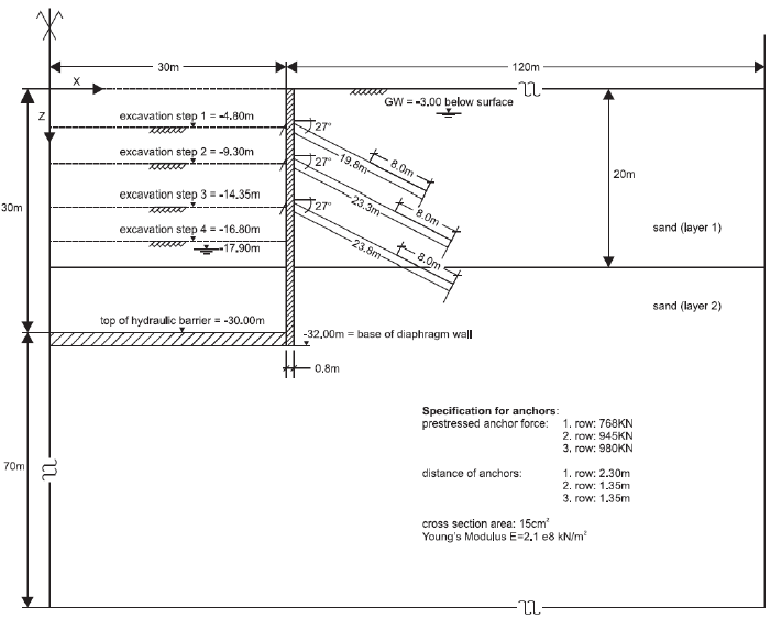
Figure 1: Geometry and excavation stages (after Schweiger, 2002).

Figure 2: Geometry and excavation stages (after Schweiger, 2002). (a) is the first font size, (b) is the second font size, and (c) is the third font size.
The analysis described by Schweiger (2002) includes nine steps:
Stage 1 – Initialize stress state, including groundwater table, 3 m below soil surface.
Stage 2 – Activate diaphragm wall and lower water level to −17.90 m in pit.
Stage 3 – Excavation step 1 (to level −4.80 m).
Stage 4 – Activate anchor row 1 at level −4.30 m and prestress anchors.
Stage 5 – Excavation step 2 (to level −9.30 m).
Stage 6 – Activate anchor row 2 at level −8.80 m and prestress anchors.
Stage 7 – Excavation step 3 (to level −14.35 m).
Stage 8 – Activate anchor row 3 at level −13.85 m and prestress anchors.
Stage 9 – Excavation step 4 (to level −16.80 m).
The zone profile and the structural elements are shown in Figure 1. The soil is modeled with the Plastic-Hardening model. The wall is model by the linear elastic zone elements. The anchors are modeled by cable structure elements.
Soil properties for the Berlin sand listed in Table 1 are adapted from Schweiger (2002).
| Parameter | Unit | Sand layer | Clay layer |
|---|---|---|---|
| dry density (\(\rho_d\)) | Mg/m3 | 1.9 | 1.9 |
| wet density (\(\rho_w\)) | Mg/m3 | 2.0 | 2.0 |
| \(E^{ref}_{50}\) | kPa | 4.5×10⁴ | 7.5×10⁴ |
| \(E^{ref}_{oed}\) | kPa | 4.5×10⁴ | 7.5×10⁴ |
| \(E^{ref}_{ur}\) | kPa | 1.8×10⁵ | 3.0×10⁵ |
| friction (\(\phi_f\)) | degrees | 35 | 38 |
| dilation (\(\psi_f\)) | degrees | 5 | 6 |
| pressure-reference (\(p_{ref}\)) | kPa | 100 | 100 |
| Poisson’s ratio (\(\nu\)) | 0.2 | 0.2 | |
| cohesion (\(C\)) | kPa | 0 | 0 |
| exponent (\(m\)) | 0.55 | 0.55 | |
| stress ratio consolidation (\(K_0\)) | 0.43 | 0.38 | |
| failure ratio (\(R_f\)) | 0.90 | 0.90 | |
| over-consolidation ratio (\(ocr\)) | 1.0 | 1.0 |
The linear elastic properties for the diaphragm wall are given in Table 2, and the anchor specifications are listed in Table 3.
| density (Mg/m3) | 2.4 |
| Young’s modulus (GPa) | 30.0 |
| Poisson’s ratio | 0.15 |
| Row 1 | Row 2 | Row 2 | |
|---|---|---|---|
| location depth ar wall (m) | 4.80 | 9.30 | 14.35 |
| dip (degree) | 27 | 27 | 27 |
| total length (m) | 19.8 | 23.3 | 23.8 |
| Anchored length (m) | 8.0 | 8.0 | 8.0 |
| spacing (m) | 2.3 | 1.35 | 1.35 |
| prestress anchor force (kN) | 768 | 945 | 980 |
| Young’s modulus (GPa) | 210 | 210 | 210 |
| cross-sectional area (m2) | 0.0015 | 0.0015 | 0.0015 |
Modeling Procedure
The FLAC3D simulation follows similar analysis stages suggested by Schweiger (2002).
Model Conditions
The Building Block tool is used to generate the grid. Zones and faces are selected, named, and densified using the Model pane. The commands resulting from both tools are exported from the State pane.
The zones close to the diaphragm wall are densified in order to refine the wall deflection
(Figure 3). The wall is separated from the rest of the mesh by using the
zone separate by-face command. Remember to use the command zone attach by-face to
attach faces after the last zone densification. The model is within a domain of \(x\) ∈ [0, 100],
\(z\) ∈ [-100, 0], and \(y\) ∈ [0, 2.7], where \(x\) = 0 denotes the symmetric plane at the
centrer of the excavation.
The roller boundary is at \(x\) = 0 to embrace the symmetry condition; the fixed boundaries are at \(z\) = -100 and \(x\) = 150 to stand for far-end conditions. No deformation is allowed in the \(y\)-axis to simulate the plane-strain condition.
The model is completed without configuring for fluid analysis. The static pore pressure is
initialized automatically by FLAC3D, provided the gravity, water density, and table information
are set using the zone water command. The soil above the water table is assigned the dry
density, while the soil below the water table is assigned the wet density.
With the pore pressures, soil densities, and the normally-consolidation coefficients available,
the stress can be conveniently initialized by the command zone initialize-stresses, the calculation of \(K_0\) from friction is performed inline.
zone initialize-stress ratio [1-math.sin(35*math.degrad)] range group 'Layer1'
zone initialize-stress ratio [1-math.sin(38*math.degrad)] range group 'Layer2'
At this stage, to set the initial stress, the exact behavior of the soil constitutive model is not
critical, so the Mohr-Coulomb model is temporarily assigned to the soil and the command
model solve elastic only is used to avoid possible uneven settlements. The data file for
this stage is “AnchoredExcavation-1.dat” and the results are stored in the file
“part-1.f3sav”.
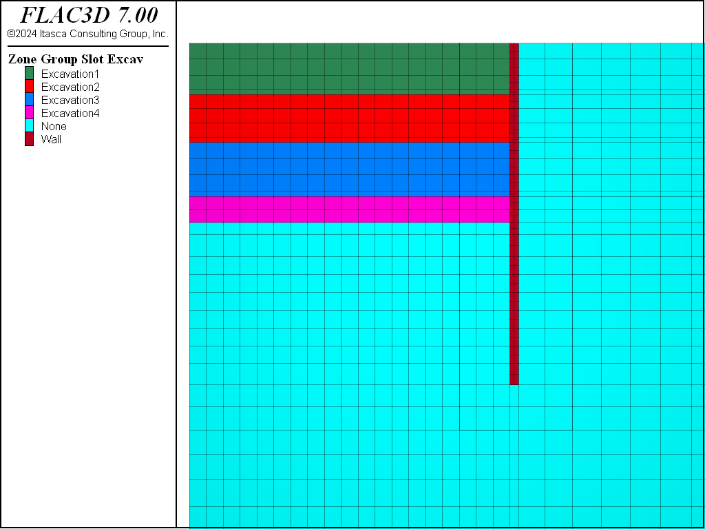
Figure 3: Model grid.
Wall Installation
The diaphragm wall activation (“AnchoredExcavation-2.dat”) is modeled by
setting the real density (2.4 Mg/m3) to the wall zones. The diaphragm wall here is modeled
by linear elastic solid zones with the properties list in Table 2.
Interface elements are assigned on the side and base surfaces of the wall to account for the
slip and separation between the wall and the soil. Note that the zone attach delete
command is used to free the boundary between the wall and the soil that was separated earlier, and
that the interface stresses are initialized using zone interface node initialize-stresses
to speed convergence. The interface friction angle is assumed to be 20°. Because the wall is heavier
than the surrounding soil, it is expected to move downward. The principal stress magnitudes and
orientations are also expected to be adjusted in the soil around the wall. The model state is
stored in the file “part-2.f3sav”.
Plastic-Hardening Model Setup
At this stage (AnchoredExcavation-3.dat), the soil models are changed to
the Plastic-Hardening model with the properties listed in Table 1.
Note that herein the Plastic-Hardening model is stress-dependent, which requires to input the
initial effective principal stress after the model is assigned the first time. This step can be
fulfilled either by zone property commands, or in this example by the following FISH
function, ini_ph.
fish def ini_ph
    loop foreach local z zone.list
        if z.model(z) = 'plastic-hardening'
            local pp   = zone.pp(z)
            zone.prop(z,'stress-1-effective') = zone.stress.min(_z) + pp
            zone.prop(z,'stress-2-effective') = zone.stress.int(_z) + pp
            zone.prop(z,'stress-3-effective') = zone.stress.max(_z) + pp
        endif
    endloop
end
This FISH function must be executed before the first cycling after the Plastic-Hardening model is assigned. Note that two parameters, constant-alpha (\(\alpha\)) and stiffness-cap-hardening (\(H_c\)), are calculated internally in this example. Users are required to check the validation of these two parameters (see Volumetric Cap Criterion and Flow Rule in the Plastic-Hardening Model definition) [ZC: please check link previous is going to correct place] before proceeding to the next stages. After equilibrium, the model state is stored in “part-3.f3sav”.
| constant-alpha | stiffness-cap-hardening | |
|---|---|---|
| Layer 1 | 1.87 | 1.07×10⁵ |
| Layer 2 | 3.23 | 6.69×10⁴ |
Dewatering
For the dewatering stage (“AnchoredExcavation-4.dat”), we assume for simplicity that the water level is dropped instantaneously within the excavation region. We start from the previous step and set the saturation, pore pressure, and permeability to zero in the current excavation area. We free the fixed pore pressure condition along the left boundary below the excavation and along the top of the model to the right of the excavation so that pore pressures can change during dewatering. We initialize the displacements in the model to zero so that we can monitor the displacement change that only occurs due to the dewatering.
When we impose a change in pore pressure, the total stress must be adjusted to account for this
change. This is done using the effective keyword in the zone water command used to
modify pore pressure.
We can check that this adjustment to total stress has been made by plotting effective stresses before and after these commands are issued: the effective stresses are unchanged in the model when the instantaneous pore pressure is imposed.
We repeat this dewatering procedure five times to account for somewhat gradual dewatering. The final pore pressure distribution is shown in Figure 4. The dewatering-induced displacement is shown in Figure 5. This indicates the amount of settlement induced by the dewatering is approximately 0.01 m. We save the model state as “part-4.f3sav” after all dewatering steps.
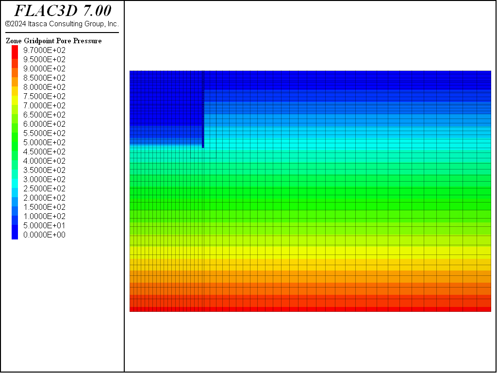
Figure 4: Pore pressure distribution following dewatering.
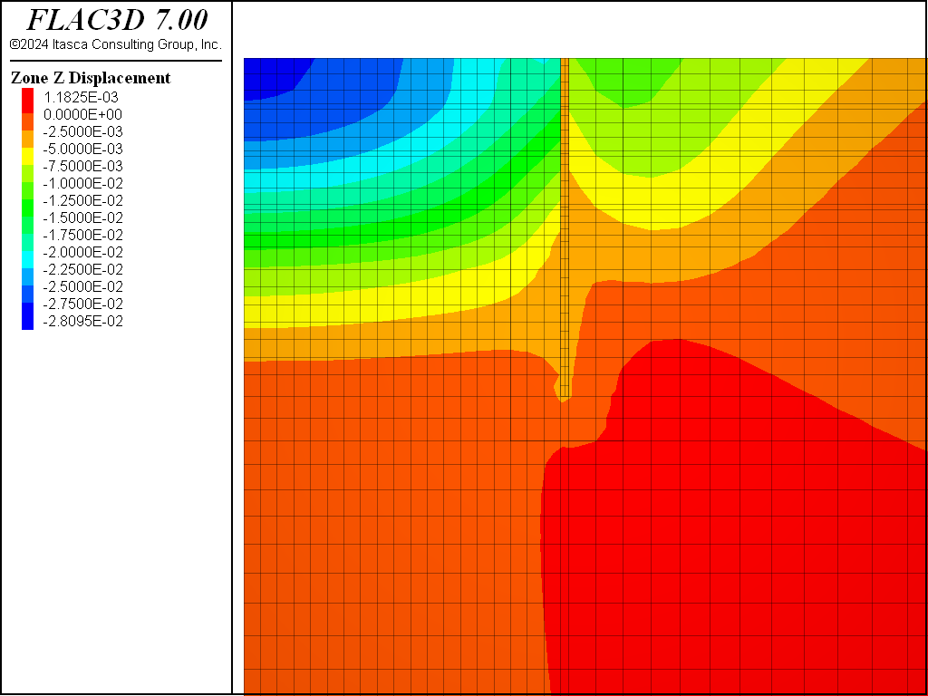
Figure 5: Displacement induced by dewatering.
Excavation and Install Anchors
Displacement is reset to zero at the start of the excavation stage. The changes in pore pressure taking place as a result of excavation are neglected in the analysis. Zones are deleted from the grid to simulate the excavation process for excavation step 1 (4.8 m depth) and the model is cycled to mechanical equilibrium (“AnchoredExcavation-5.dat”). The displacement induced by excavation to a depth of 4.8 m is plotted in Figure 6.
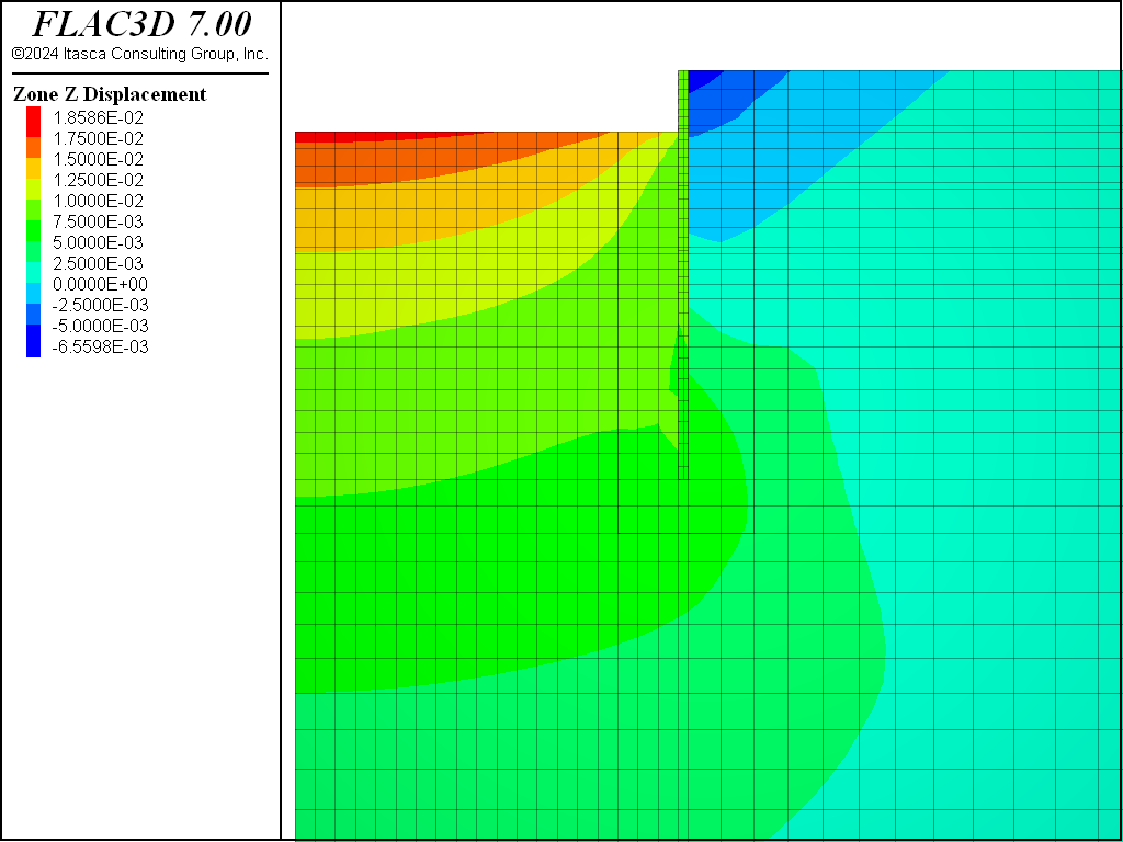
Figure 6: Displacement induced by excavation to a depth of 4.8 m.
A cable structural element 19.8 m long is installed at the excavation step 1 level at a dip of 27°
(“AnchoredExcavation-6.dat”). The top end of the cable is attached to the
wall, and the last 8 m are anchored to the soil (the shear bond strength is 100 MPa). The anchor is
prestressed with a force of 901.6 kN, which has been adjusted from the original prestress anchor
force (768 kN) by a factor of 2.7/2.3, where 2.7 m is the model out-of-plane width, and 2.3 m is
the distance of anchors at row 1 (see specification in Figure 1). The
pretensioning is performed using the structure cable apply tension command, whereby (1) the
tension is applied to the ungrouted section of the cable; (2) the model is solved to equilibrium;
and (3) the tension on the cable is freed to adjust naturally from then on. Figure 7 plots the axial anchor forces after pretesioning of the first row anchor.
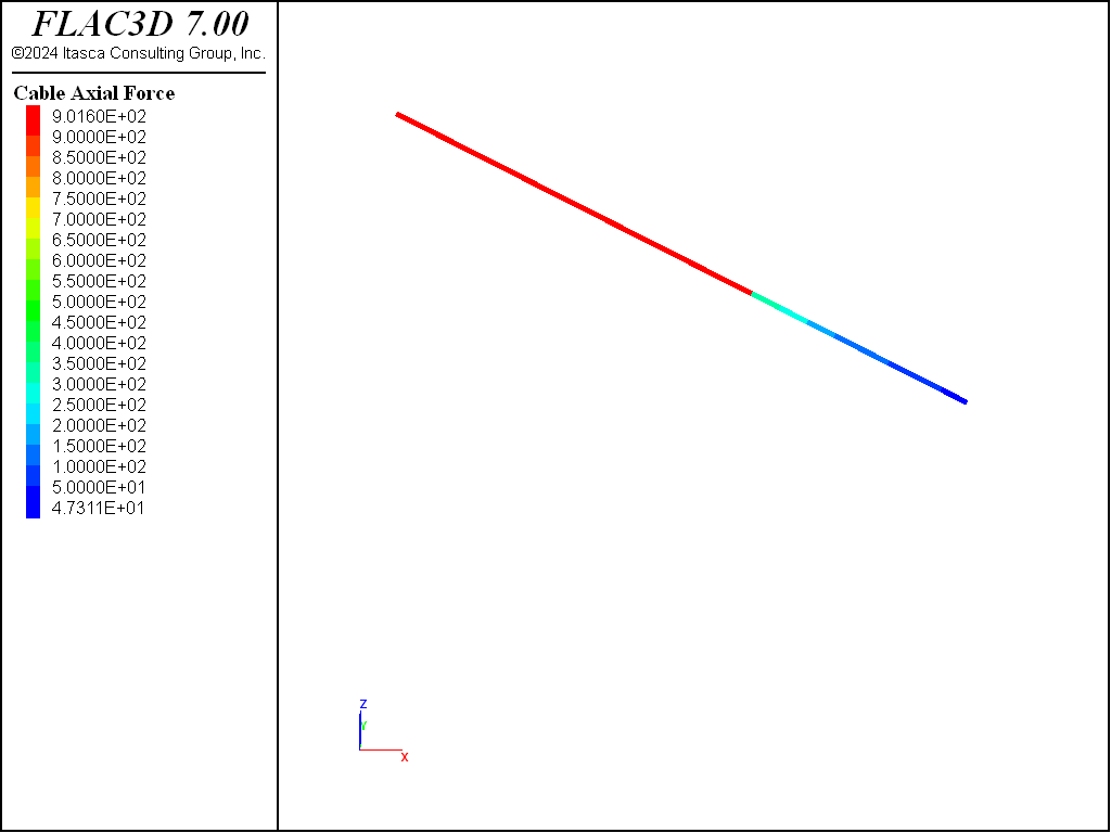
Figure 7: Axial forces in anchor to a depth of 4.8 m after pretensioning.
Zones are then removed from the grid to a depth of 9.3 m, and the model is cycled to mechanical equilibrium (“AnchoredExcavation-7.dat”). The displacement induced by excavation to 9.3 m depth is plotted in Figure 8.
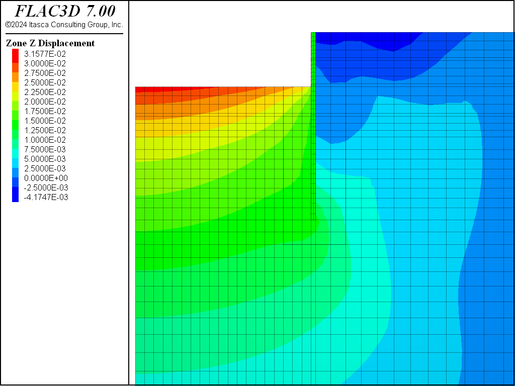
Figure 8: Displacement induced by excavation to a depth of 9.6 m.
The second row of anchors 23.3 m in length are now installed and prestressed with a 945 kN force in the same manner (“AnchoredExcavation-8.dat”). Figure 9 plots the axial anchor forces after pretesioning of anchor row 2.
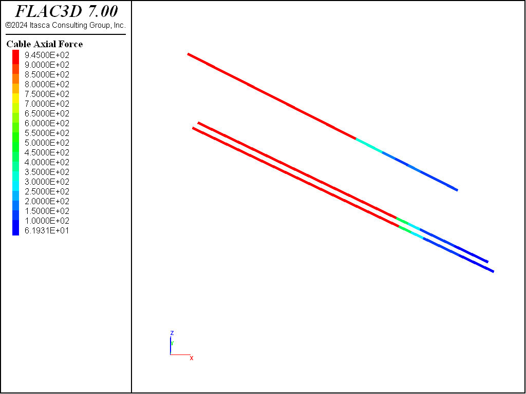
Figure 9: Axial forces in anchor at a depth of 9.6 m after pretensioning.
Zones are then removed for the excavation to 14.35 m depth, and the model is cycled to equilibrium again (“AnchoredExcavation-9.dat”). The displacement induced by excavation to a depth of 14.35 m is plotted in Figure 10.
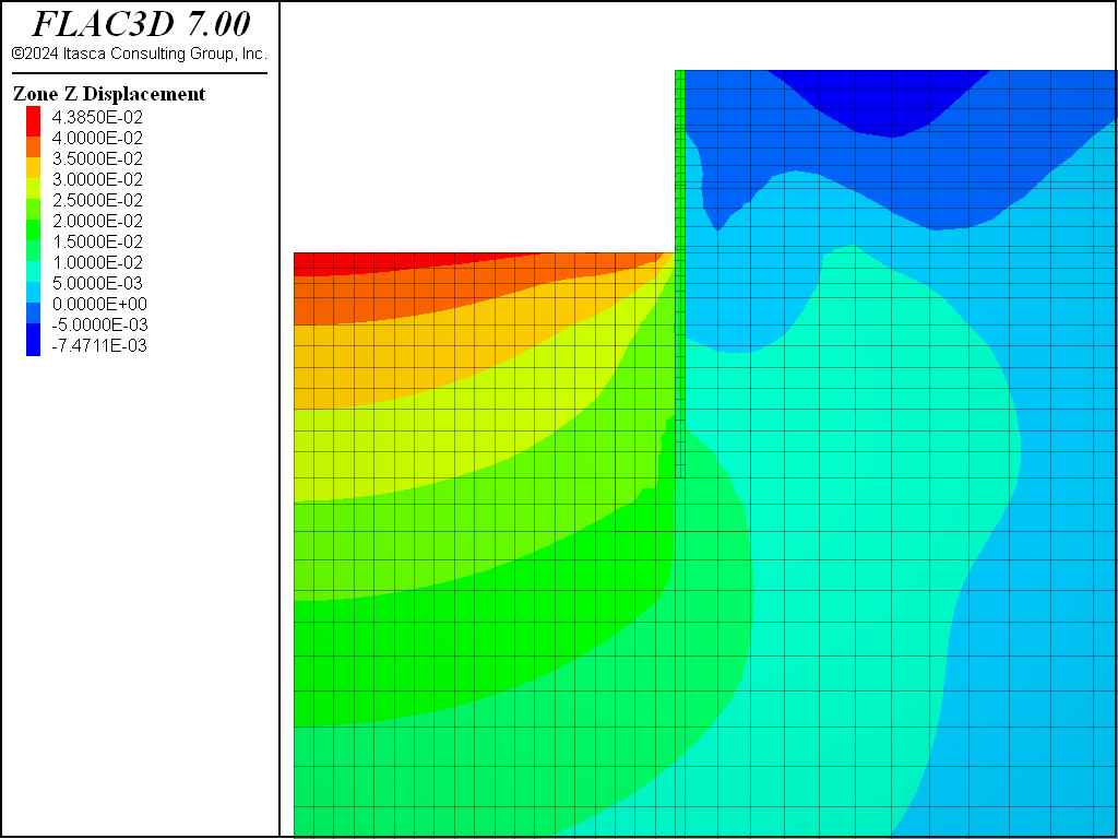
Figure 10: Displacement induced by excavation to a depth of 14.35 m. .
The procedure is repeated once more for the third row of anchors 23.8 m in length with a 980 kN prestress force (“AnchoredExcavation-10.dat”), and excavation to the final depth of 16.8 m (“AnchoredExcavation-11.dat”). After the third row anchors, the axial anchor forces are plotted in Figure 11, and the displacement induced by excavation to a depth of 14.35 m is plotted in Figure 12.
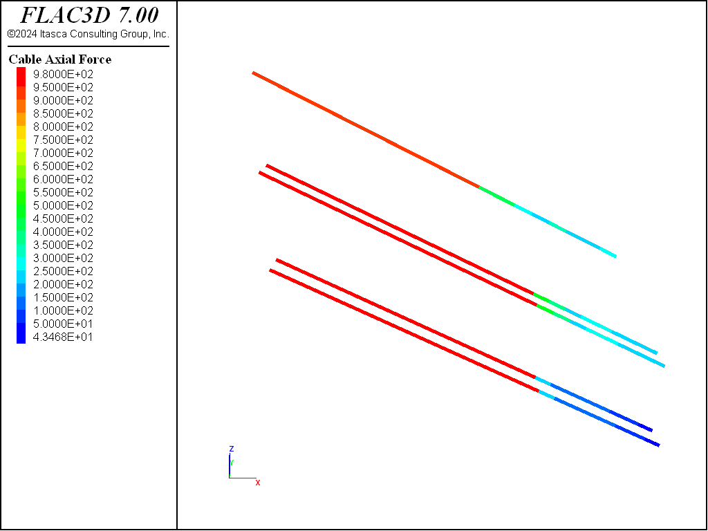
Figure 11: Axial forces in anchor to a depth of 13.45 m after pretensioning.
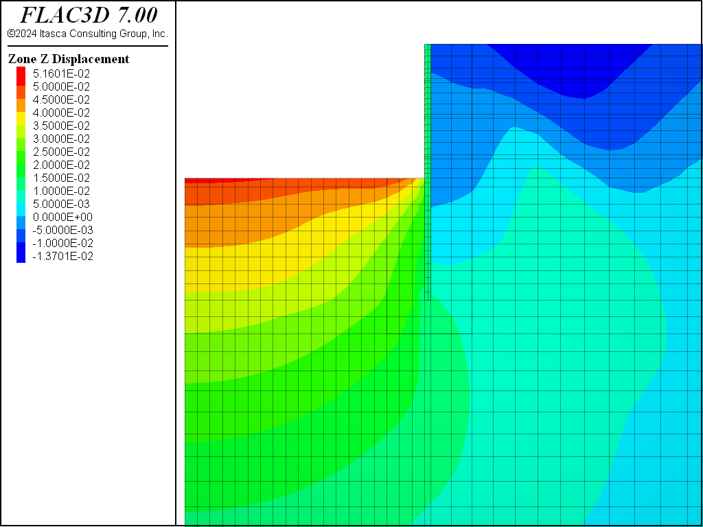
Figure 12: Displacement induced by excavation to 14.35 m depth.
The calculated wall deflection after the final excavation step are compared to the measured values in Figure 13.
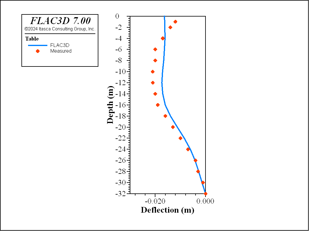
Figure 13: Measured wall deflection and FLAC3D calculation.
The calculated ground settlement behind the wall is presented in Figure 14. It is notable that the calculated ground settlement curve behind the wall is mainly downward, which is consistent with the geotechnical observations.
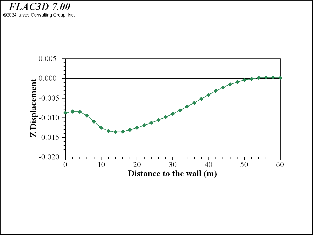
Figure 14: Calculated ground settlement behind the wall.
References
Schweiger, HF. “Results from numerical benchmark exercises in geotechnics,” in 5th European Conference Numerical Methods in Geotechnical Engineering, Vol. 1, pp. 305–314. Presses de l’ENPC/LCPC, Paris (2002).
Data Files
AnchoredExcavation-1.dat
model new
model large-strain off
model title "Anchored Excavation"
; Model creation
program call 'geometry' suppress ; Created interactive with Building Blocks,
                         ; exported from State Pane
zone generate from-building-blocks
program call 'names' suppress ; Zones named and densified with Model Pane,
                      ; exported from State Pane
zone face skin ; Name model boundaries
zone separate by-face clear-attach ...
     range group 'WallLeft' or 'WallRight' or 'WallBottom' ; Separate wall
                                                           ; zones ahead of
                                                           ; time
zone attach by-face   ; Attach densified and separated zones
; Install gravity and fluid properties
model grav 10 ; m/s^2
zone water density 1 ; Mg/m^3
zone water plane origin (0,0,-3) norm (0,0,-1)
; Assign initial constitutive model and properties
zone cmodel assign mohr-coulomb
zone property young 1.8e5 poisson 0.2 friction 35 dilation 5 ...
              cohesion 1 range group 'Layer1' ; kPa
zone property young 3.0e5 poisson 0.2 friction 38 dilation 6 ...
              cohesion 1 range group 'Layer2' ; kPa
; Set wet and dry densities
zone property density 1.9 range group 'Dry'
zone property density 2.0 range group 'Wet'
; Roller boundaries on sides, fixed on bottom and right
;zone face apply velocity-normal 0 range group 'South' or 'North'
zone face apply velocity-normal 0 range group 'South' or 'North'
zone face apply velocity-normal 0 range group 'West2'
zone face apply velocity (0,0,0) range group 'East2' or 'Bottom3'
; Initialize stress, with different ratios in the layers
zone initialize-stress ratio [1-math.sin(35*math.degrad)] range group 'Layer1'
zone initialize-stress ratio [1-math.sin(38*math.degrad)] range group 'Layer2'
;
zone history name 'disp' displacement-x position (30,0,0)
; Solve
model solve convergence 1
;
model save 'part-1'
AnchoredExcavation-2.dat
model restore 'part-1'
; Reset displacements so we can track changes from last state
zone gridpoint initialize displacement (0,0,0)
; Separate wall by removing attach conditions
zone attach delete range group 'WallLeft' or 'WallRight' or 'WallBottom'
; Create side and bottom interfaces separately
zone interface name 'side' create by-face ...
                                  range group 'WallLeft' or 'WallRight'
zone interface name 'bot' create by-face range group 'WallBottom'
zone interface node property stiffness-shear 8e6 stiffness-normal 8e6 ...
                             friction 20.0
; Initialize stresses on the interface to accelerate convergence
zone interface node initialize-stress
;
model solve convergence 1
; Change the density and stiffness of the wall
zone cmodel assign elastic                     range group 'Wall'
zone prop density 2.4 young 3.0e7 poisson 0.15 range group 'Wall'
; Relax the convergence criteria in the very stiff wall,
; and in the zones around it at the top.
zone gridpoint initialize ratio-target 1e-2 ...
                          range position-x 28 33 position-z -4.8 0
zone gridpoint initialize ratio-target 1e-2 range group 'Wall'
;
model solve convergence 1
;
model save 'part-2'
AnchoredExcavation-3.dat
model restore 'part-2'
; Reset displacements to track incremental changes from each part.
zone gridpoint initialize displacement (0,0,0)
; Assign plastic hardening model and properties to layers.
zone cmodel assign plastic-hardening range group 'Wall' not
zone property pressure-ref 100 poisson 0.2 failure-ratio 0.9 cohesion 1
zone property stiffness-50-reference 7.5e4 stiffnes-ur-reference 3.0e5 ...
              stiffness-oedometer-reference 7.5e4 ...
              range group 'Layer2' group 'Wall' not
zone property stiffness-50-reference 4.5e4 stiffness-ur-reference 1.8e5 ...
              stiffness-oedometer-reference 4.5e4 ...
              range group 'Layer1' group 'Wall' not
zone property exponent 0.55 friction 35 dilation 5 ...
              over-consolidation-ratio 1 ...
              range group 'Layer1' group 'Wall' not
zone property exponent 0.55 friction 38 dilation 6 ...
              over-consolidation-ratio 1 ...
              range group 'Layer2' group 'Wall' not
zone property coefficient-normally-consolidation ...
              [1-math.sin(35*math.degrad)] ...
              range group 'Layer1' group 'Wall' not
zone property coefficient-normally-consolidation ...
              [1-math.sin(38*math.degrad)] ...
              range group 'Layer2' group 'Wall' not
; Initialize effective stress properties using FISH.
fish operator ini_ph(z)
    if z.model(z) = 'plastic-hardening'
        local pp   = zone.pp(z)
        zone.prop(z,'stress-1-effective') = zone.stress.min(z) + pp
        zone.prop(z,'stress-2-effective') = zone.stress.int(z) + pp
        zone.prop(z,'stress-3-effective') = zone.stress.max(z) + pp
    endif
end
[ini_ph(::zone.list)])
; Get to approximate equilibrium
model solve convergence 1
;
model save 'part-3'
AnchoredExcavation-4.dat
model restore 'part-3'
; Reset displacements to track incremental changes from each part.
zone gridpoint initialize displacement (0,0,0)
; Clear pore-pressures in the wall
zone gridpoint initialize pore-pressure 0 range group 'Wall'
; Dewater in 5 steps, gradually lowering the water table
; (keeping effective stress constant)
; First step
zone water plane origin (0,0,-6) normal (0,0,1) effective ...
     range group 'Left' position-z -30 0
zone property density 1.9 range group 'Left' position-z -6 0
model solve convergence 1
; Second step
zone water plane origin (0,0,-9) normal (0,0,1) effective ...
     range group 'Left' position-z -30 0
zone property density 1.9 range group 'Left' position-z -9 0
model solve convergence 1
; Third step
zone water plane origin (0,0,-12) normal (0,0,1) effective ...
     range group 'Left' position-z -30 0
zone property density 1.9 range group 'Left' position-z -12 0
model solve convergence 1
; Fourth step
zone water plane origin (0,0,-15) normal (0,0,1) effective ...
     range group 'Left' position-z -30 0
zone property density 1.9 range group 'Left' position-z -15 0
model solve convergence 1
; Fifth step
zone water plane origin (0,0,-17.9) normal (0,0,1) effective ...
     range group 'Left' position-z -30 0
zone property density 1.9 range group 'Left' position-z -17.9 0
model solve convergence 1
;
model solve convergence 1
;
model save 'part-4'
AnchoredExcavation-5.dat
; excavate to -4.80 m
model restore 'part-4'
; Reset displacements to track incremental changes from each part.
zone gridpoint initialize displacement (0,0,0)
; Delete zones in excavation, solve, and save.
zone delete range group 'Excavation1'
zone history name 'disp2' displacement-x position (30,0,0)
model solve convergence 1
model save 'part-5'
AnchoredExcavation-6.dat
model restore 'part-5'
; This creates geometry representing the cable layout,
; could also just be imported from CAD.
program call 'cablegeom' suppress
; Create and set properties for grouted and ungrouted first cable set
struct cable import from-geometry 'cable' offset (0,1.35,0) ...
       group 'free1' id 1 range group 'free1'
struct cable import from-geometry 'cable' offset (0,1.35,0) ...
       group 'grout1' segments 8 id 1 range group 'grout1'
struct cable prop young 2.1e8 cross-section-area 0.00176 ...
                  grout-stiffness 0    grout-cohesion 0  ...
                  grout-perimeter 0.15 range group 'free1'
struct cable prop young 2.1e8 cross-section-area 0.00176  ...
                  grout-stiffness 4e6  grout-cohesion 1e5 ...
                  grout-perimeter 0.15 range group 'grout1'
; Connect first node of cable with the zone rigidly
struct link delete range group 'free1' position-x 30.4
struct link create target zone range group 'free1' position-x 30.4
; Pretension the cable, adjust to equilibrium, then free
; the cable tension to adjust naturally.
struct cable apply tension value 901.6 range group 'free1'
model solve convergence 1
struct cable apply tension active off
;
model save 'part-6'
AnchoredExcavation-7.dat
model large-strain off
; excavate to -9.30 m
model rest 'part-6'
;
zone delete range group 'Excavation2'
model solve convergence 1
;
model save 'part-7'
AnchoredExcavation-8.dat
model restore 'part-7'
; Create and set properties for grouted and ungrouted second cable set
struct cable import from-geometry 'cable' offset (0,0.675,0) ...
       group 'free2'             id 2 range group 'free2'
struct cable import from-geometry 'cable' offset (0,0.675,0) ...
       group 'grout2' segments 8 id 2 range group 'grout2'
struct cable import from-geometry 'cable' offset (0,2.025,0) ...
       group 'free2'             id 2 range group 'free2'
struct cable import from-geometry 'cable' offset (0,2.025,0) ...
       group 'grout2' segments 8 id 2 range group 'grout2'
struct cable prop young 2.1e8 cross-section-area 0.0015   ...
                  grout-stiffness 0    grout-cohesion 0   ...
                  grout-perimeter 0.1373 range group 'free2'
struct cable prop young 2.1e8 cross-section-area 0.0015   ...
                  grout-stiffness 4e6  grout-cohesion 1e5 ...
                  grout-perimeter 0.1373 range group 'grout2'
; Connect first node of cable with the zone rigidly
struct link delete range group 'free2' position-x 30.4
struct link create target zone range group 'free2' position-x 30.4
; Pretension the cable, adjust to equilibrium,
; then free the cable tension to adjust naturally.
struct cable apply tension value 945 range group 'free2'
model solve convergence 1
struct cable apply tension active off
;
model save 'part-8'
AnchoredExcavation-9.dat
model large-strain off
; excavate to -14.35 m
model rest 'part-8'
;
zone delete range group 'Excavation3'
model solve convergence 1
;
model save 'part-9'
AnchoredExcavation-10.dat
model restore 'part-9'
; Create and set properties for grouted and ungrouted second cable set
struct cable import from-geometry 'cable' offset (0,0.675,0) ...
       group 'free3'             id 3 range group 'free3'
struct cable import from-geometry 'cable' offset (0,0.675,0) ...
       group 'grout3' segments 8 id 3 range group 'grout3'
struct cable import from-geometry 'cable' offset (0,2.025,0) ...
       group 'free3'             id 3 range group 'free3'
struct cable import from-geometry 'cable' offset (0,2.025,0) ...
       group 'grout3' segments 8 id 3 range group 'grout3'
struct cable prop young 2.1e8 cross-section-area 0.0015    ...
                  grout-stiffness 0    grout-cohesion 0    ...
                  grout-perimeter 0.1373 range group 'free3'
struct cable prop young 2.1e8 cross-section-area 0.0015    ...
                  grout-stiffness 4e6  grout-cohesion 1e5  ...
                  grout-perimeter 0.1373 range group 'grout3'
; Connect first node of cable with the zone rigidly
struct link delete range group 'free3' position-x 30.4
struct link create target zone range group 'free3' position-x 30.4
; Pretension the cable, adjust to equilibrium,
; then free the cable tension to adjust naturally.
struct cable apply tension value 980 range group 'free3'
model solve convergence 1
struct cable apply tension active off
;
model save 'part-10'
AnchoredExcavation-11.dat
model large-strain off
; excavate to -16.8 m
model rest 'part-10'
;
zone delete range group 'Excavation4'
model solve convergence 1
;
model save 'part-11'
| Was this helpful? ... | PFC © 2021, Itasca | Updated: Feb 25, 2024 |