
Hopper Flow
Introduction
Note
The project file for this example may be viewed/run in PFC.[1] The data files used are shown at the end of this example.
This example demonstrates the use of PFC to model the discharge of spherical particles from a hopper. A simple hopper discharge model is presented in the hopper tutorial. In that case, a cylindrical hopper is utilized. In the present example, periodic boundaries are used to reduce the influence of the hopper geometry. The effects of friction and fill height are investigated via a parametric study; they are shown to have a significant influence on the hopper discharge rate and flow patterns. This example is based on the work from [Anand2008] and [Ketterhagen2009].
Numerical Model
The hopper is created and filled by the FISH function build_hopper defined in “hopper_utilities.dat”. To efficiently create the initial system, the brick logic is used. Bricks are ball andor clump specimens built in periodic space. Walls cannot be present in bricks. As a result, one can place bricks adjacent to one another so that they fit together perfectly without the introduction of forces due to overlap.
The hopper geometry is shown in Figure 1. The depth of the model in the periodic direction is set to five times the average particle diameter. The hopper dimensions in the \(x\)- and \(z\)-directions are also set to be multiples of the average particle diameter.
The wall generate polygon command is used to generate the hopper geometry. Care must be taken when model components span the entire domain in the periodic direction. In this case, contacts may not form between the large object and the objects that have been periodically placed. As a result, walls must be decomposed into multiple facets in the periodic direction to avoid such situations.
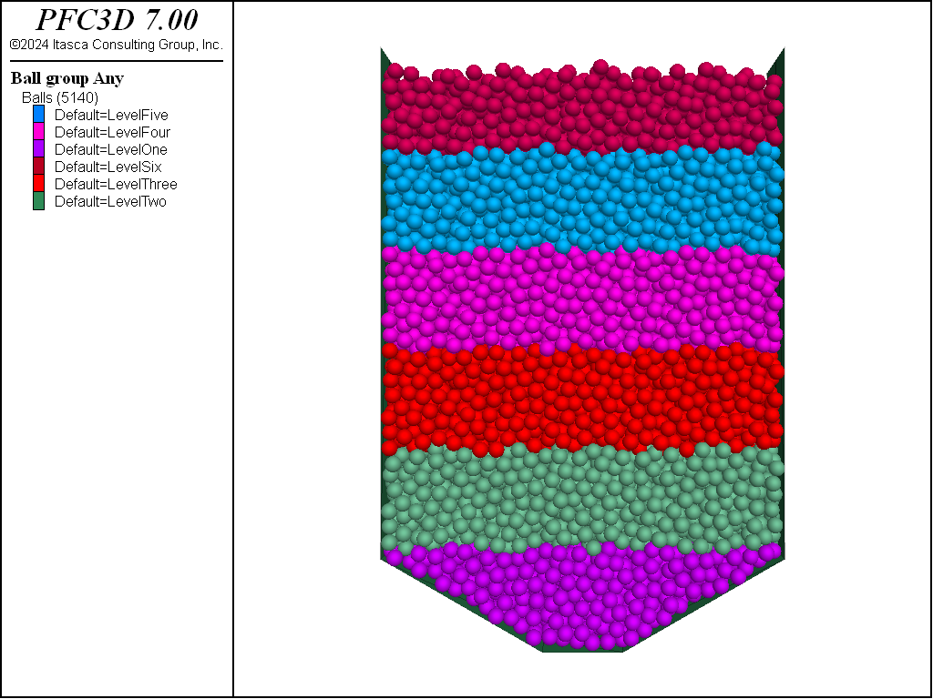
Figure 1: Filled hopper where groups are assigned to delineate horizontal layers.
Simulation of Hopper Discharge
Use the Action FISH function to undertake a discharge experiment.
fish define Action(fill_level,key)
  z_min = fill_level*H / 100.0
  z_max = 2*H
  command
    ball delete range position-z [z_min] [z_max]
  endcommand
  discharged_mass = 0
  filename = 'fill_'+string(int(fill_level))+'_'+key
  command
model cycle 5000 calm 50
model solve ratio-average 1e-3
    ball attribute damp 0.0
    wall delete range set id 1001 1002
    model mechanical time-total 0.0
    model mechanical timestep auto
    model results interval mechanical 0.1 prefix [key]
    wall results active true
    ball results add-attribute velocity active true
    fish callback add MeasureDischargedMass event ball_delete
    program echo off
model solve fish-halt HaltControl
    program echo on
    fish callback remove MeasureDischargedMass event ball_delete
    model save [filename]
  endcommand
end
The hopper can be filled to varying levels depending on the fill_level argument. Balls above the desired fill_level are deleted, and the system is equilibrated. Local damping is then set to zero (see the ball attribute command) for the discharge portion of the simulation, the bottom cap is removed and the mechanical age is reset to zero (see the model mechanical time-total command). Before discharge is initiated, the ball results command is used to periodically record reduced versions of the model state. In this example, the ball group identifiers and velocities are recorded along with the ball locations and radii.
The discharged mass is measured during the simulation via registering a FISH function with a callback event (see the fish callback command). As balls hit the negative \(z\)-domain boundary, they are deleted due to the condition set with the model domain command. The FISH function MeasureDischargedMass is registered with the ball_delete event. Whenever a ball is deleted, this FISH function is executed with the ball pointer provided as the argument. In this way, the mass of each deleted ball can be accumulated. A table is filled containing the discharged mass as a function of mechanical time.
fish define MeasureDischargedMass(bp)
    global discharged_mass
    discharged_mass = discharged_mass + ball.mass.real(bp)
    command
        table [filename] insert [mech.time.total] [discharged_mass]
    endcommand
end
The simulation stops when few balls remain, using the model solve fish-halt command. This allows one to connect a FISH function to the solve logic so that cycling will continue until the specified criteria are met. In order for cycling to cease, the FISH function must return a nonzero value. A value is returned by a FISH function when a value is assigned to the FISH function name. For instance, the statement HaltControl = temp assigns the return value. Once the solve limit has been reached, a table containing the discharged mass as a function of time is exported to a .tab file for further scrutiny (see the table export command).
fish define HaltControl
  local temp = 0
  if ball.num < 5
    command
      table [filename] export [filename]
    endcommand
    temp = 1
  endif
  HaltControl = temp
end
Repeated Simulation
The “hopper_doall.dat” data file performs the hopper discharge simulations with varying parameters of interest. More precisely, the hopper discharge is repeated while varying the friction coefficient (we will refer to the high friction and the low friction cases) and the height to which the hopper is filled. The influence of these parameters on the type of particle flow (e.g., mass flow versus funnel flow) and on the mass discharge rate can be investigated.
Figures 2 and 3 show the flow patterns during discharge for the low and high friction cases, respectively. The patterns are qualitatively different, transitioning from mass-flow to funnel flow with increasing friction.
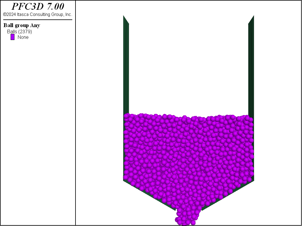
Figure 2: Homogeneous mass flow pattern resulting from low friction.
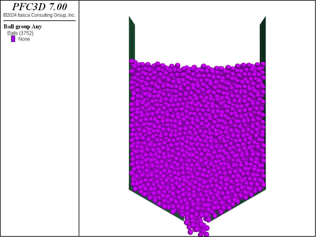
Figure 3: Funnel flow pattern resulting from high friction.
Figures 4 and 5 show the evolution of the discharge rate for two fill levels in the low and high friction cases, respectively. The blue lines represent the completely filled hopper; the green lines correspond with the hopper filled to half its total height. For the low friction case, the discharge rate increases with increasing fill height. With a larger friction coefficient, the discharge rate is relatively independent of fill height. These findings are consistent with the results of [Anand2008] and [Ketterhagen2009].
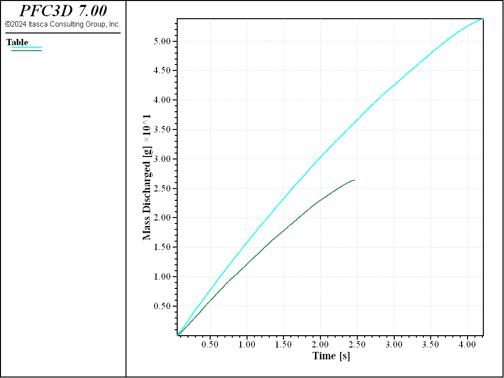
Figure 4: Mass discharged from a hopper versus time, low friction coefficient case. The value of the mass discharge rate strongly depends on the filling height (blue line—completely filled, green line—half filled) of the hopper.
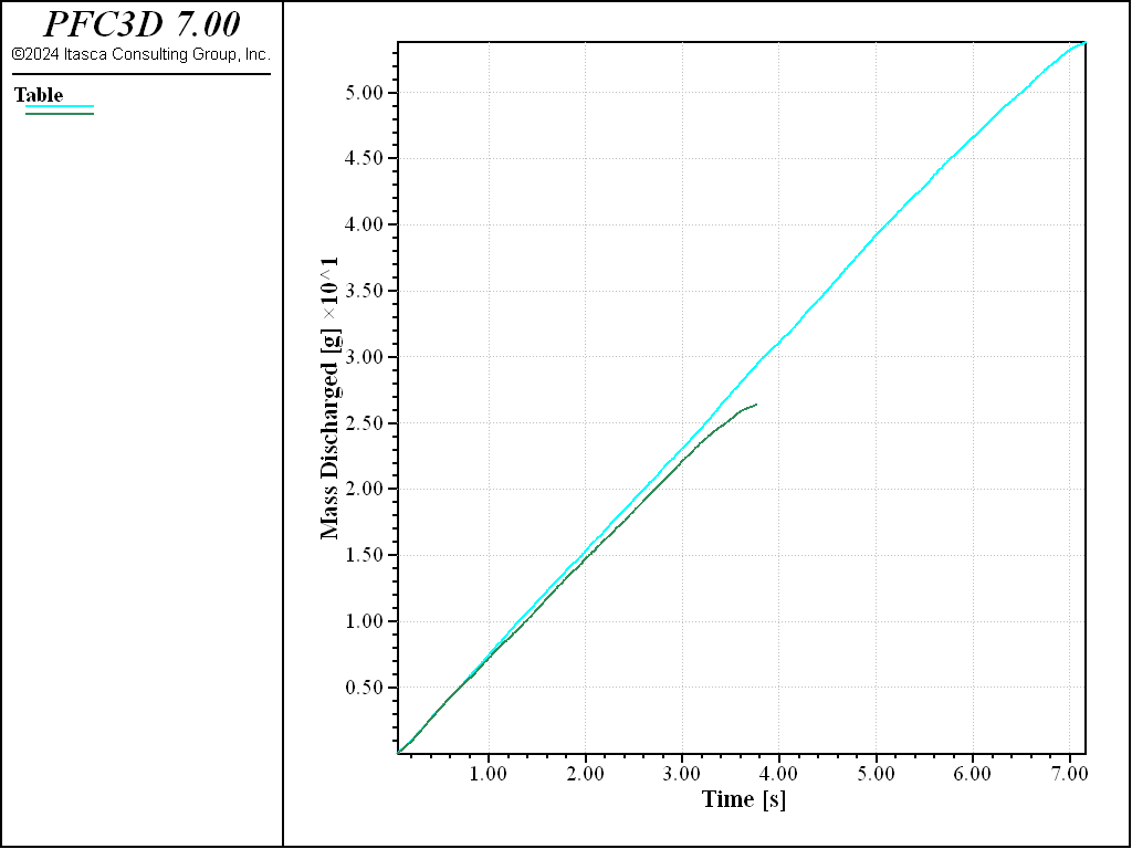
Figure 5: Mass discharged from a hopper versus time, high friction coefficient case. The influence of the fill height (blue line—completely filled, green line—half filled) on the mass discharge rate is small.
Making a Movie of the Simulation
As described above, the ball results command has been utilized to save reduced states of the model periodically. These result files can be used effectively to post-process the simulation, allowing one to visualize the evolution of the system. In addition, as the balls are recreated, one can rerun analyses using the FISH functions similar to those used during the simulation. A series of images may also be created. The function makeMovie defined in “hopper_utilities.dat” illustrates how this can be achieved.
fish define makeMovie(fname)
    global rmap
    command
        model result map rmap
    endcommand
    cnt = 1
    loop foreach local res rmap
        local str = string.build("%1%2.png",fname,cnt)
        cnt = cnt + 1
        command
            model result import [res] skip-fish
            plot export bitmap filename [str]
        endcommand
    endloop
end
The images can then be assembled into a movie using third-party tools.
Discussion
This example illustrates several important aspects of using PFC to undertake a parametric investigation. Custom solve limits and FISH function executions resulting from the occurrences of callback events are used to manage the simulations and collect pertinent data. Without such tools, it would be very difficult to undertake a study of this nature.
References
| [Anand2008] | (1, 2) Anand A., Curtis J.S., Wassgren C.R., Hancock B.C., Ketterhagen W.R. “Predicting discharge dynamics from a rectangular hopper using the discrete element method (DEM),” in Chemical Engineering Science, Vol. 63, pp. 5821-5830, 2008. |
| [Ketterhagen2009] | (1, 2) Ketterhagen W.R., Curtis J.S., Wassgren C.R., Hancock B.C., “Predicting the flow mode from hoppers using the discrete element method,” in Powder Technology, Vol. 195, pp. 1-10, 2009. |
Data Files
hopper_doall.dat
; fname: Hopper_doall.p3dat
;
; Granular flow from a rectangular hopper.
; The effects of hopper friction and particle friction are investigated,
; and shown to have a significant influence on the hopper discharge behaviour
;============================================================================

model new
program call 'Hopper_utilities' suppress

;------------ LOW FRICTION CASE
[build_hopper(0.05,0.01,30.0)]
model save 'hopper_ini'
[Action(50,'LowFriction1')]
model restore 'hopper_ini'
[Action(100,'LowFriction2')]
model save 'LowFrictionHopper'

;------------HIGH FRICTION
model restore 'hopper_ini'
ball property 'fric' 0.8
wall property 'fric' 0.8
[Action(50,'HighFriction1')]
model restore 'hopper_ini'
ball property 'fric' 0.8
wall property 'fric' 0.8
[Action(100,'HighFriction2')]
model save 'HighFrictionHopper'

;==============================================================================
; eof: Hopper_doall.p3dat
hopper_utilities.dat
model large-strain on
; fname: Hopper_utilities.p3dat
;
; Utilities for hopper simulation
; ============================================================================

fish define build_hopper(fric,brad,theta)
  local cfric = fric
  ;
  ballRadius = brad
  W0 = ballRadius*10
  W = W0*5.0
  H = W*1.50
  d = ballRadius*5.0
  B = (W-W0)*0.5
  theta = 30*math.pi/180
  A = B*math.tan(Theta)
  command
    ; build a brick
    model domain condition periodic
    model domain extent ([-W/4],[W/4]) ([-d], [d]) (0,[W/4])
    contact cmat default model linear ...
                 property kn 1e4 ks 5e3 fric [cfric] dp_nratio 0.2
    contact cmat default type ball-facet model linear ...
        property kn 1.5e4 ks 7.5e3 fric [cfric] dp_nratio 0.2

    ball distribute bin 1 radius [ballRadius]
    ball attribute density 2500 damp 0.7
model cycle 1000 calm 10
    model mechanical timestep scale
model solve
    brick make id 1
    ; delete existing balls, build the hopper and assemble the brick
    ball delete
    model domain condition destroy periodic destroy
    model domain extent ([-W/2],[W/2]) ([-d],[d]) ([-d],[H*2.0])

    wall generate group 'leftlateral_1'  polygon ...
         ([-W/2],[-d],[A]) ([-W/2],0.0,[A]) ([-W/2],[-d],[H]) ([-W/2],0.0,[H])
    wall generate group 'leftlateral_2'  polygon ...
         ([-W/2],0.0,[A]) ([-W/2],[d],[A]) ([-W/2],0.0,[H]) ([-W/2],[d],[H])
    wall generate group 'rightlateral_1' polygon ...
         ([W/2],[-d],[A]) ([W/2],0.0,[A]) ([W/2],[-d],[H]) ([W/2],0.0,[H])
    wall generate group 'rightlateral_2' polygon ...
         ([W/2],0.0,[A]) ([W/2],[d],[A]) ([W/2],0.0,[H]) ([W/2],[d],[H])
    wall generate group 'leftbottom_1'   polygon ...
         ([-W0/2],[-d],0.) ([-W0/2],0.0,0.0) ([-W/2],[-d],[A]) ([-W/2],0.0,[A])
    wall generate group 'leftbottom_2'   polygon ...
         ([-W0/2],0.0,0.0) ([-W0/2],[d],0.0) ([-W/2],0.0,[A]) ([-W/2],[d],[A])
    wall generate group 'rightbottom_1'  polygon ...
         ([W0/2],[-d],0.0) ([W0/2],0.0,0.0) ([W/2],[-d],[A]) ([W/2],0.0,[A])
    wall generate group 'rightbottom_2'  polygon ...
         ([W0/2],0.0,0.0) ([W0/2],[d],0.0) ([W/2],0.0,[A]) ([W/2],[d],[A])

    wall generate id 1001 group 'cap' polygon ...
         ([-W0/2],[-d],0) ([W0/2],[-d],0.0) ([-W0/2],0.0,0.0) ([W0/2],0.0,0.0)
    wall generate id 1002 group 'cap' polygon ...
        ([-W0/2],0.0,0.0) ([W0/2],0.0,0.0) ([-W0/2],[d],0.0) ([W0/2],[d],0.0)

    brick assemble id 1 origin ([-W/2],[-d],0.0) size 2 1 6
    ball delete range plane origin ([-W0/2],0.0,0.0) ...
         dip  30.0 dip-direction 90.0 below
    ball delete range plane origin ([ W0/2],0.0,0.0) ...
         dip -30.0 dip-direction 90.0 below
    ball attribute density 2500 damp 0.7
    model clean
    [trim]
    model gravity 0 0 -9.81
    model history name '1' mech ratio-average
model cycle 1000 calm 100
model solve ratio-average 1e-3
    ball group 'LevelOne' range position-z 0.0 [H/6]
    ball group 'LevelTwo' range position-z [H/6][2*H/6]
    ball group 'LevelThree' range position-z [2*H/6][3*H/6]
    ball group 'LevelFour' range position-z [3*H/6][4*H/6]
    ball group 'LevelFive' range position-z [4*H/6][5*H/6]
    ball group 'LevelSix' range position-z [5*H/6][2*H]
  endcommand
end

fish define trim
  loop foreach local c contact.list('ball-facet')
    local bp = contact.end1(c)
    ball.delete(contact.end1(c))
  endloop
end

; excerpt-wnro-start
fish define MeasureDischargedMass(bp)
    global discharged_mass
    discharged_mass = discharged_mass + ball.mass.real(bp)
    command
        table [filename] insert [mech.time.total] [discharged_mass]
    endcommand
end
; excerpt-wnro-end


; excerpt-prpp-start
fish define HaltControl
  local temp = 0
  if ball.num < 5
    command
      table [filename] export [filename]
    endcommand
    temp = 1
  endif
  HaltControl = temp
end
; excerpt-prpp-end

; excerpt-yurt-start
fish define Action(fill_level,key)
  z_min = fill_level*H / 100.0
  z_max = 2*H
  command
    ball delete range position-z [z_min] [z_max]
  endcommand
  discharged_mass = 0
  filename = 'fill_'+string(int(fill_level))+'_'+key
  command
model cycle 5000 calm 50
model solve ratio-average 1e-3
    ball attribute damp 0.0
    wall delete range set id 1001 1002
    model mechanical time-total 0.0
    model mechanical timestep auto
    model results interval mechanical 0.1 prefix [key]
    wall results active true
    ball results add-attribute velocity active true
    fish callback add MeasureDischargedMass event ball_delete
    program echo off
model solve fish-halt HaltControl
    program echo on
    fish callback remove MeasureDischargedMass event ball_delete
    model save [filename]
  endcommand
end
; excerpt-yurt-end

; excerpt-qonr-start
fish define makeMovie(fname)
    global rmap
    command
        model result map rmap
    endcommand
    cnt = 1
    loop foreach local res rmap
        local str = string.build("%1%2.png",fname,cnt)
        cnt = cnt + 1
        command
            model result import [res] skip-fish
            plot export bitmap filename [str]
        endcommand
    endloop
end
; excerpt-qonr-end

;==============================================================
; eof: Hopper_utilities.p3dat
Endnotes
| [1] | To view this project in PFC, use the program menu.
⮡ PFC |
| Was this helpful? ... | PFC © 2021, Itasca | Updated: Feb 25, 2024 |