
Balls in a Box
Introduction
Note
The project file for this example may be viewed/run in PFC.[1] The data files used are shown at the end of this example.
This simple example models 30 balls interacting in a box. Gravity is activated, and the system is cycled to a target age limit twice:
- once with no energy dissipation, and
- once with energy dissipation via frictional slip and viscous damping at the contacts.
This example demonstrates basic usage of the ball generate, ball attribute, and contact cmat default commands and makes use of the linear contact model. A similar tutorial demonstrating the creation of clumps in a box is given in the “Clumps in a Box” section.
Numerical Model
The complete data file (3D) for this example is “cmlinear_simple.dat (3D)”. Select lines of this file are discussed below. Since the command structure is identical for PFC3D and PFC2D, this data file will operate with the latter as well (only the number of balls generated will differ).
The first three lines of the file—discounting lines starting with a semicolon ( ; ), which are comments that are ignored for command/FISH processing—call the model new command, set the model to calculate in large strain mode (see Large Strain/Small Strain), and set the job title for this project.
model new
model large-strain on
model title 'Balls in a box'
Issuing a model new command clears the entire model and is useful if you run the file multiple times or when previous operations have been performed. The large- or small-strain calculation mode can be set at any time prior to cycling. Most PFC models will run in large strain mode; the command to turn on large strain mode is usually found at or near the very beginning of the model. The job title is empty by default. Note that the job title may also be set using the General Options dialog under the menu.
Next, the extent of the domain is specified using the model domain command.
model domain extent -10.0 10.0
It is necessary to define the domain extent before any model components can be created. PFC uses this information for geometric calculations and contact detection (see the “Domain” section for details). This command sets the domain extent to be a cubic box with a side length of 20.0 units centered on the origin of the model (always at (0.0,0.0,0.0)). Here this is achieved by specifying the edges of the extent in the \(x\)-direction only. When the extent edges in the \(y\)- and/or \(z\)-direction(s) are not specified, the extent edges of the preceding direction are used. Also note that domain conditions (i.e., conditions to be applied when a model component reaches the domain boundaries) can be specified with the model domain command. The stop condition is the default, which sets to 0 the translational and angular velocities of model components whose centroids reach a domain boundary.
Next, the contact cmat default command is used to select the default mechanical contact model to be installed by PFC whenever a new contact is created. Here the linear contact model is selected. One can also specify contact model properties with the property keyword. In this case, the normal stiffness of 1.0e6 stiffness units is specified.
contact cmat default model linear property kn 1.0e6
This command operates on the Contact Model Assignment Table (CMAT). Contact detection occurs while cycling, and the list of contacts is updated based on the proximity of pieces to one another (refer to the “Cycling” section for a detailed description of the cycle sequence). The contact detection scheme also deletes contacts if the pieces move far enough from one another that they no longer interact. Whenever a contact is created, the CMAT is queried to select the appropriate contact model to install. At program start-up, the CMAT contains default slots for each contact type (e.g., ball-ball, ball-facet, etc.) that are filled with the Null contact model. This means that, by default, bodies will not interact or “see” each other. The contact cmat default command is used to modify these default slots. If no contact type is specified, then all default slots are modified. Note that the CMAT may contain additional entries (each associated with a specific range), which easily permits building complex mechanical behaviors into the system, as discussed in the tutorial example “Using the CMAT”. Please refer to this tutorial and to “contact cmat commands” for further details.
The next three lines are used to generate 30 balls in a cubic box composed of wall facets.
wall generate box -5.0 5.0 ;one-wall
model random 10001
ball generate radius 1.0 1.4 box -5.0 5.0 number 30
The wall generate command creates a cubic box with sides of length 10.0 units centered about the origin of the model. The syntax for repetition of extent edges is similar to the domain specification described above. The one-wall keyword may be given to force all generated facets to belong to the same wall, as opposed to creating one wall for each face of the box. Other predefined shapes (e.g., cylinders, spheres, etc.) may be generated with the wall generate command. A wall is always a collection {of line segments in 2D; triangular facets in 3D}. It is also possible to create a wall and its facets using the wall create command or to import a wall from an existing STL or DXF file in 3D, or from a geometry object in 2D or 3D, using the wall import command.
Balls are generated using the ball generate command: 30 balls with radii ranging from 1.0 to 1.4 units are created in a box the size of the wall. Notice that there are no initial overlaps since the ball generate command generates balls that fall completely within the specified box. The ball centroids are positioned randomly within the box and the radii are chosen randomly from a uniform distribution by default. This behavior can be modified by using additional keywords of the ball generate command. Notice also that the model random command is issued prior to generating the balls to fix the seed of the random number generator internally used by PFC. This algorithm actually corresponds to a pseudo random number generator, which is capable of generating sequences of random numbers starting from a seed number, which are reproducible if the seed number is fixed. In practice, this means that the exact same model is created anytime the file is executed, as long as the seed number is fixed. The ball generate command produces a specimen where balls do not overlap. Other commands may be used to create balls (such as the ball create command, which creates a single ball, or the ball distribute command, which produces a specimen with a target porosity without regard to overlap).
The next line uses the ball attribute command to assign the density of the balls.
ball attribute density 100.0
PFC requires balls to have a nonzero density in order to resolve ball equations of motion. An error occurs at the beginning of a cycle sequence if a ball with zero density exists. The ball attribute command can be used to set all attributes of the balls. Note that the term attribute has a very specific meaning in PFC and is fundamentally different from a property. This distinction is discussed in the tutorial example “Attributes and Properties.”
Gravity is set with the model gravity command.
model gravity 10.0
Using the syntax above, gravity will be assumed to act in the {minus \(y\)-direction in 2D; minus \(z\)-direction in 3D}. Gravity may be oriented arbitrarily if all components of the gravity vector are specified (see model gravity for details).
At this stage, the model is ready to be solved. Before proceeding, the model save command is used to save the current state of the system to “initial-state.sav”.
model save 'initial-state'
Note that the model state (SAV) file extension is automatically appended to the file name if no extension is specified by the user.
The system is then cycled with the model solve command with a target time limit of 10.0 time units, and the resulting state is saved.
model solve time 10.0
model save 'caseA-nodamping'
The model solve command is used to initiate and continue cycling until a target limit criterion is reached. Alternatively, the model cycle command can be used to perform a given number of cycles.
As no energy dissipation mechanisms were introduced in the model, the total energy initially present in the form of potential energy is conserved and distributed into potential, kinetic, and elastic strain energy partitions. Figure 1 shows the state of the system with balls colored by velocity magnitude. As one can see, a high level of agitation remains in the system.
Note
This response would not be observed, by default, in PFC version 4.0 or earlier due to the default local damping coefficient of 0.7. In PFC version 5.0 or later, though, there is no local damping by default (one can set the local damping coefficients with the ball attribute damp, clump attribute damp and rblock attribute damp commands).
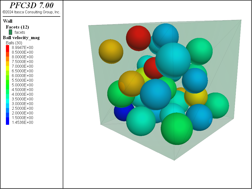
Figure 1: The system after cycling (case A - no energy dissipation).
The initial system is then restored with the model restore command.
model restore 'initial-state'
Similar to the model save command, a SAV file extension is automatically assumed if not specified in the command.
The CMAT is modified to introduce energy dissipation into the system.
contact cmat default model linear property ...
                                  kn 1.0e6 ks 1.0e6 fric 0.25 dp_nratio 0.1
The linear contact model continues to be used as the default model, though the properties are changed to activate friction and viscous damping in the normal direction. Please refer to the linear contact model description for details of the model and the contact model properties.
Modifying the CMAT does not alter existing contacts, because their contact models have already been assigned. Contacts created after the CMAT modification will be affected. To modify existing contacts, the contact cmat apply command is used.
contact cmat apply
This command forces the CMAT to be queried for all existing contacts and reassigns the contact model. Using this command results in the deletion of all information previously stored in the contact model, and should be used with care. Alternatively, “contact commands” can be used to modify the contact model or properties at select existing contacts.
Finally, the system is solved to the target time limit and a new SAV file is created.
model solve time 10.0
model save 'caseB-damping'
Figure 2 shows the state of the system: balls have settled on the floor of the box.
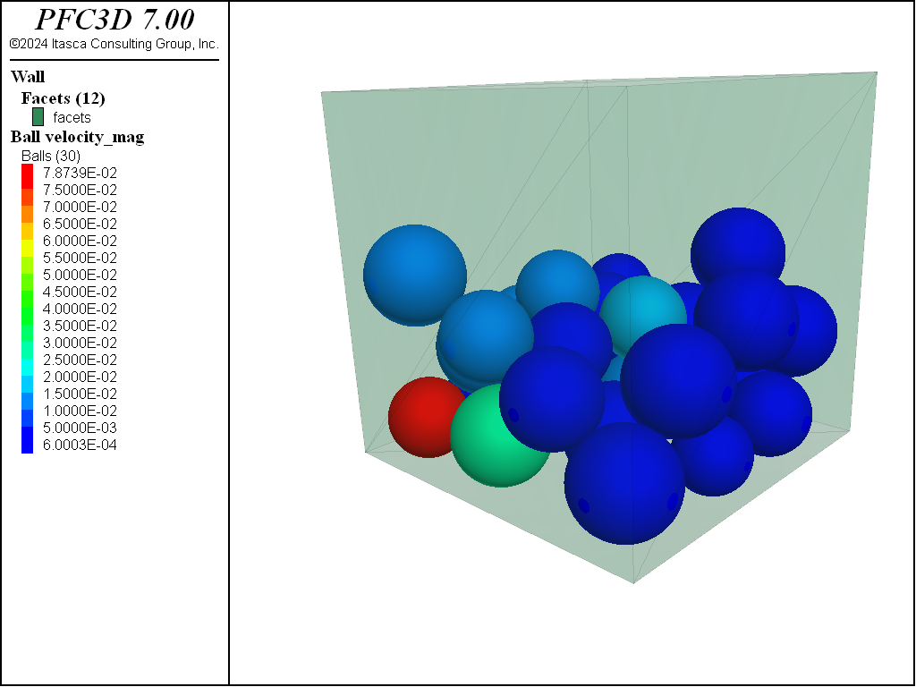
Figure 2: The system after cycling (case B - energy dissipation activated).
Discussion
This tutorial introduces the main steps required to build a simple PFC model. They can be summarized as follows.
- Define the domain extent;
- Define the CMAT;
- Generate the initial state;
- Perform alterations and solve the system; and, possibly,
- Repeat step 4 to conduct sensitivity analyses.
Important PFC features, concepts, and commands have been discussed for each step. The user is encouraged to visit the detailed descriptions of these topics in the corresponding sections of the documentation.
Data Files
cmlinear_simple.dat (3D)
; fname: cmlinear_simple.dat (3D)
;
;  Exercise the Linear contact model
;=============================================================================
; excerpt-mrls-start
model new
model large-strain on
model title 'Balls in a box'
; excerpt-mrls-end

; Set the domain extent
; excerpt-lrls-start
model domain extent -10.0 10.0
; excerpt-lrls-end

; Modify the default slots of the Contact Model Assignment Table
; Here we choose the linear contact model (with kn=1e6) for all contact types
; excerpt-arqq-start
contact cmat default model linear property kn 1.0e6
; excerpt-arqq-end

; Generate 30 balls in a box
; excerpt-lkmk-start
wall generate box -5.0 5.0 ;one-wall
model random 10001
ball generate radius 1.0 1.4 box -5.0 5.0 number 30
; excerpt-lkmk-end

; Assign ball density
; excerpt-pipp-start
ball attribute density 100.0
; excerpt-pipp-end

; Activate gravity
; excerpt-iorr-start
model gravity 10.0
; excerpt-iorr-end

;Save the initial state
; excerpt-nmxx-start
model save 'initial-state'
; excerpt-nmxx-end

; Solve for a given time and save the model
; excerpt-ljjz-start
model solve time 10.0
model save 'caseA-nodamping'
; excerpt-ljjz-end

; Restore the initial state
; excerpt-xdso-start
model restore 'initial-state'
; excerpt-xdso-end

; Modify the default slots of the Contact Model Assignement Table
; Newly created contacts will use these settings
; excerpt-pejs-start
contact cmat default model linear property ...
                                  kn 1.0e6 ks 1.0e6 fric 0.25 dp_nratio 0.1
; excerpt-pejs-end
; Apply the CMAT to existing contacts as well
; Note that the contact model will be overridden (and therefore all previous
; information will be lost)
; excerpt-ueew-start
contact cmat apply
; excerpt-ueew-end

; Solve for a given time and save the model
; excerpt-rnsm-start
model solve time 10.0
model save 'caseB-damping'
; excerpt-rnsm-end

program return
;=============================================================================
; eof: cmlinear_simple.dat (3D)
cmlinear_simple.dat (2D)
; fname: cmlinear_simple.dat (2D)
;
;  Exercise the Linear contact model
;=============================================================================
model new
model large-strain on
model title 'Balls in a box'

; Set the domain extent
model domain extent -10.0 10.0

; Modify the default slots of the Contact Model Assignment Table
; Here we choose the linear contact model (with kn=1e6) for all contact types
contact cmat default model linear property kn 1.0e6

; Generate 30 balls in a box
wall generate box -5.0 5.0 one-wall
model random 10001
ball generate radius 1.0 1.5 box -4.0 4.0 number 30

; Assign ball density
ball attribute density 100.0

; Activate gravity
model gravity 10.0

;Save the initial state
model save 'initial-state'

; Solve for a given time and save the model
model solve time 10.0
model save 'caseA-nodamping'

; Restore the initial state
model restore 'initial-state'

; Modify the default slots of the Contact Model Assignement Table
; Newly created contacts will use these settings
contact cmat default model linear property ...
                                  kn 1.0e6 ks 1.0e6 fric 0.25 dp_nratio 0.1
; Apply the CMAT to existing contacts as well
; Note that the contact model will be overridden (and therefore all previous
; information will be lost)
contact cmat apply

; Solve for a given time and save the model
model solve time 10.0
model save 'caseB-damping'

program return
;=============================================================================
; eof: cmlinear_simple.dat (2D)
Endnotes
| [1] | To view this project in PFC, use the program menu.
⮡ PFC |
| Was this helpful? ... | PFC © 2021, Itasca | Updated: Feb 25, 2024 |