
Hertz Contact Model: Complex Loading Paths
Problem Statement
Note
The project file for this example may be viewed/run in PFC.[1] The data files used are shown at the end of this example.
The Hertz Model provides a nonlinear elastic force-displacement law, with viscous dashpots. The purpose of this example is to analyze the response of a single contact under complex loading paths. Results for a ball-ball contact and a ball-wall interaction are discussed and compared.
PFC3D Models
Two simple systems are set up. The first system is composed of two identical balls of unit diameter; in the second system, the bottom ball is replaced with a circular wall.
All degrees of freedom are fixed for both bodies in contact, and the top ball is displaced in order to load the contact, with the following loading path (in the global coordinate system):
- Normal loading for \(t\) = 0.1 [time-unit] (loading displacement along \(\mathbf{Y}\))
- Rolling for \(t\) = 0.05 [time-unit] (rotation around \(\mathbf{Z}\))
- Rolling for \(t\) = 0.05 [time-unit] (rotation around \(\mathbf{X}\))
- Twisting for \(t\) = 0.05 [time-unit] (rotation around \(\mathbf{Y}\))
- Normal unloading for \(t\) = 0.1 [time-unit] (unloading displacement along \(\mathbf{Y}\))
For both systems, the same loading path is repeated three times, with a different set of properties as follows (refer to the “Hertz Model” section for a detailed description and listing of the properties):
- \(G\) = 1.0 × 10⁹, \(\nu\) = 0.3, and \(\mu\) = 0.5.
- Same as 1. with \(M_s\) = 1 (activate scaling down of the shear force upon normal unload).
- Same as 2. with \(\beta_n=\beta_s= 0.5\) and \(M_d\) = 1 (activate viscous damping).
Model Results
Ball-Ball Contact

Figure 1: Ball-ball contact model at the end of loading stage 1a.
Two identical balls with unit diameter are submitted to the loading paths detailed above. Fig. 1 shows the state of the system at the end of loading stage 1a (normal loading). In this figure, the contact is represented twice: as a line perpendicular to the contact plane, and as a disk coplanar with the contact plane.
The histories of the magnitude of the normal and shear forces (both in the springs and the dashpots) monitored during loading 1, 2, and 3 are shown in Figs. 2 to 4, respectively.
The evolution of the normal force in the spring is identical in all three cases: it increases non-linearly during normal loading stage a), maintains a constant value during rolling and twisting loading stages b), c), and d), then vanishes non-linearly during normal unloading stage e). Its maximal value, which corresponds to an overlap of 1.0 × 10⁻³ [length-unit], agrees with the analytical solution of 3.0117 × 10⁴ [force-unit] given by equation (3) and (4) in the Hertz contact model description [SE: verify the link and reference in the preceding are correct].
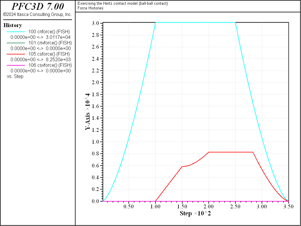
Figure 2: Evolution of the spring and dashpot forces (normal and shear) during loading path 1. Ball-ball contact.

Figure 3: Evolution of the spring and dashpot forces (normal and shear) during loading path 2. Ball-ball contact.
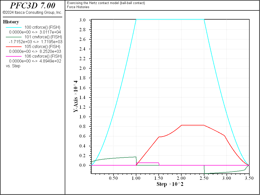
Figure 4: Evolution of the spring and dashpot forces (normal and shear) during loading path 3. Ball-ball contact.
The evolution of the shear force in the spring is identical for cases 2) and 3), but differs for case 1) due to the different value of \(M_s\). In case 1), the shear force remains null during normal loading stage a), then increases linearly during rolling loading stage b). During the latter, the slope is given by the initial tangent shear stiffness, which is constant at constant overlap (equation (11) in the Hertz contact model description). [SE: verify the link and reference in the preceding are correct] During rolling stage c), the magnitude of the shear force increases non-linearly, although the overlap does not change (thus the initial tangent shear stiffness). This is because the loading direction changed, and the shear force is now made up of two components (along the \(\mathbf{X}\) and \(\mathbf{Z}\) global axes). The shear force magnitude is not affected by twisting (loading stage d)), because no shear displacement is built up during this stage. However, the direction of the shear force vector accommodates the relative twist between the balls, as shown in Fig. 5, where the absolute value of the \(x\)-component of the shear force decreases linearly, while the absolute value of the \(z\)-component of the shear force increases linearly during the twisting loading stage (mechanical time from 0.2 to 0.25 [time-unit]). Finally, because no shear displacement is built up during the normal unloading stage 1e), the shear force remains constant at the beginning of this stage (Fig. 2, mechanical time from 0.25 to \(\approx 0.28\) [time-unit]). However, as the unloading proceeds, the Coulomb slip criterion is eventually met, and the shear force vanishes with the normal force (mechanical time from \(\approx 0.28\) to 0.35 [time-unit]).
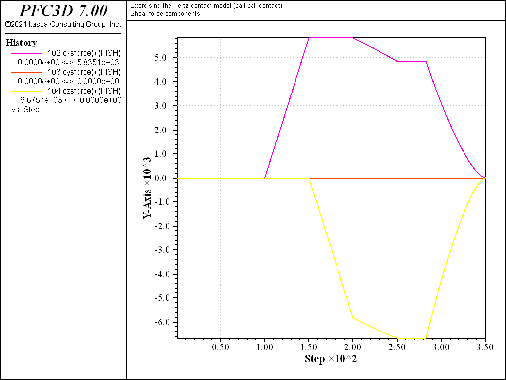
Figure 5: Evolution of the spring shear force components during loading path 1. Ball-ball contact.
The evolution of the shear force in cases 2) and 3) is similar to that of case 1), except during the normal unloading stage e). For those cases, scaling-down of the shear force upon normal unload is activated (\(M_s\) = 1). Thus the shear force starts decreasing linearly while the normal force is decreasing, until the Coulomb criterion is met and the shear force vanishes proportionally to the normal force (Fig. 2, mechanical time from 0.25 to 0.35 [time-unit]). Because the shear force magnitude at the beginning of slip is therefore lower in cases 2) and 3) than in case 1), the energy dissipated during sliding will also be lower. This can be seen by comparing Figs. 6, 7, and 8, which show the evolution of the contact energies (strain energy and slip and dashpot work) during loading cases 1), 2), and 3), respectively. Note that viscous damping is activated only for loading case 3), which is the only case where the dashpot forces (Fig. 4) and dashpot work (Fig. 6) are nonzero.
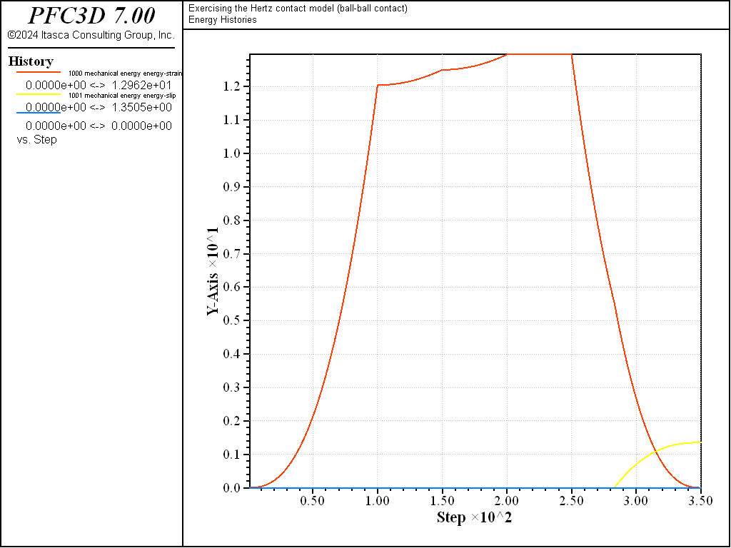
Figure 6: Evolution of the contact energies (strain energy, slip work, and dashpot work) during loading path 1. Ball-ball contact.
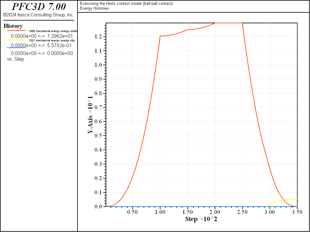
Figure 7: Evolution of the contact energies (strain energy, slip work, and dashpot work) during loading path 2. Ball-ball contact.
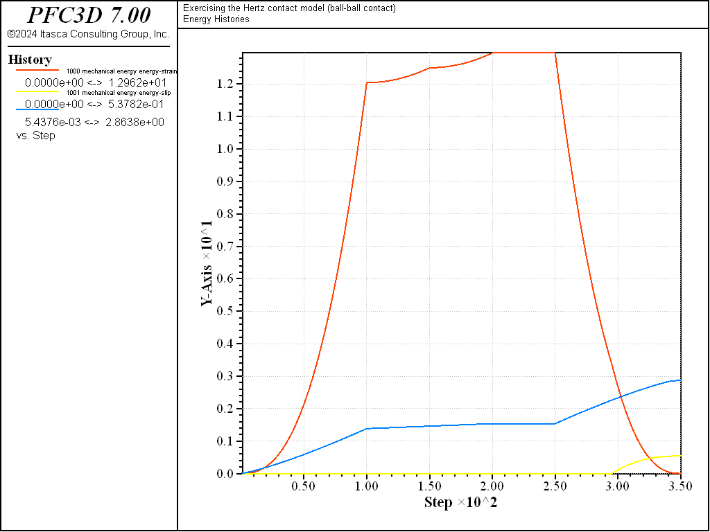
Figure 8: Evolution of the contact energies (strain energy, slip work, and dashpot work) during loading path 3. Ball-ball contact.
Ball-Wall Interaction
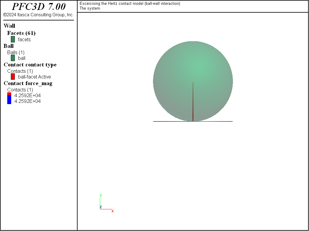
Figure 9: Ball-wall interaction model at the end of loading stage 1a.
Fig. 9 shows the state of the system at the end of loading stage 1a (normal loading), for the ball-wall interaction case. In this case, multiple contacts exist between the ball and the facets that make up the wall. However, since full contact resolution mode is active (default setting), only one contact is deemed active at a time, although more than one contact may exhibit a positive overlap (refer to the description of the faceted wall logic for further details).
The histories of the magnitude of the normal and shear forces (both in the springs and the dashpots) monitored during loading 1, 2, and 3 are shown in Figs. 10 to 12 respectively, and the histories of the contact energies are shown in Figs. 13 to 15.
All quantities evolve qualitatively similarly to the ball-ball contact case. However, they are quantitatively different, although the contact shear modulus \(G\) and Poisson ratio \(\nu\) are identical, because the contact effective radius is different (equation (6) in the Hertz contact model description [SE: verify the link and reference in the preceding are correct]).
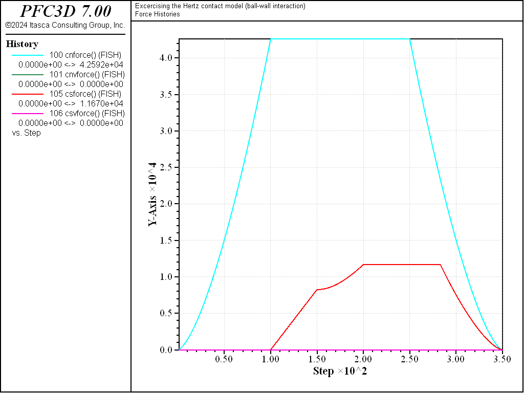
Figure 10: Evolution of the spring and dashpot forces (normal and shear) during loading path 1. Ball-facet contact.

Figure 11: Evolution of the spring and dashpot forces (normal and shear) during loading path 2. Ball-facet contact.
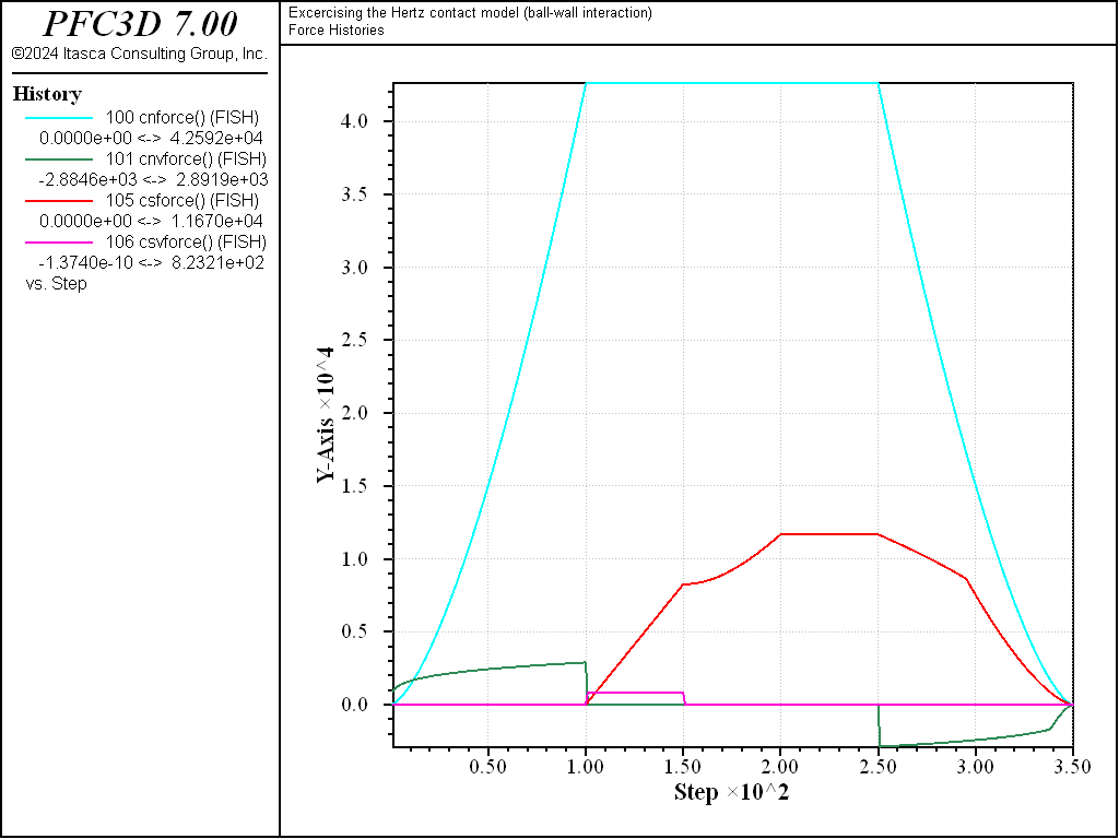
Figure 12: Evolution of the spring and dashpot forces (normal and shear) during loading path 3. Ball-facet contact.
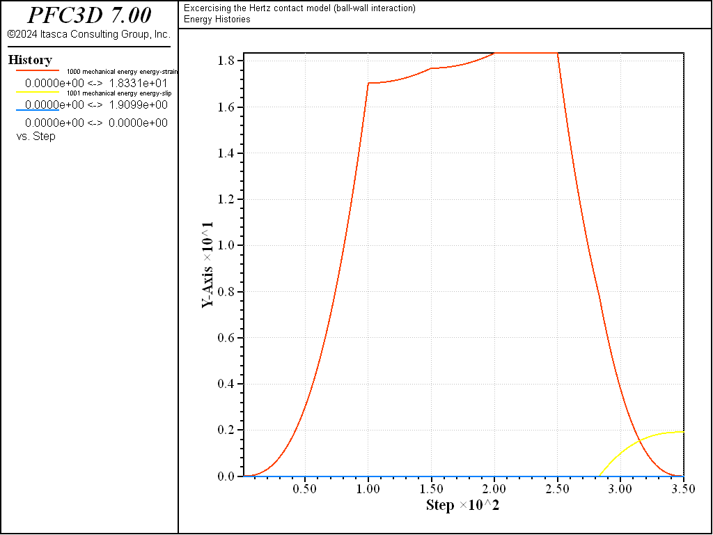
Figure 13: Evolution of the contact energies (strain energy, slip work, and dashpot work) during loading path 1. Ball-facet contact.
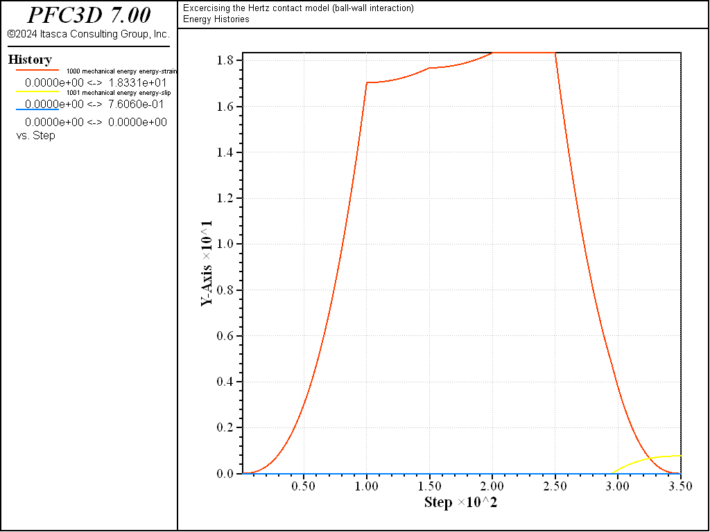
Figure 14: Evolution of the contact energies (strain energy, slip work, and dashpot work) during loading path 2. Ball-facet contact.
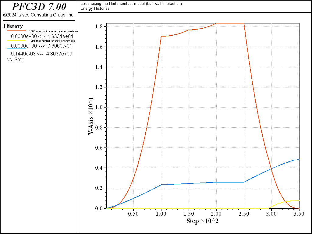
Figure 15: Evolution of the contact energies (strain energy, slip work, and dashpot work) during loading path 3. Ball-facet contact.
Conclusion
In this example, a ball-ball contact and a ball-wall interaction with the Hertz contact model are exercised under complex loading paths. The evolution of the forces and energies are discussed and compared.
Data Files
cmhertz-setup.dat (3D)
model large-strain on
; fname: cmhertz-setup.p3dat
;     Setup shared parameters, loading path and history monitoring
; =============================================================================

model domain extent -2 2 -2 2 condition periodic
contact cmat default model hertz property hz_shear 1e9 hz_poiss 0.3 fric 0.5
model mechanical timestep fix 1e-3

fish define monitor
  modeltime = mech.time.total
  cnforce = 0
  cnvforce = 0
  csforce = 0
  csvforce = 0
  loop foreach local cp contact.list
    hz_f_loc = contact.prop(cp,'hz_force')
    cnforce  = comp.x(hz_f_loc)
    hz_fs_loc = hz_f_loc
    comp.x(hz_fs_loc) = 0.0
    csforce  = math.mag(hz_fs_loc)
    hz_fs_glob = contact.to.global(cp,hz_fs_loc)
    cxsforce  = comp.x(hz_fs_glob)
    cysforce  = comp.y(hz_fs_glob)
    czsforce  = comp.z(hz_fs_glob)
    cnvforce = comp.x(contact.prop(cp,'dp_force'))
    csvforce = comp.y(contact.prop(cp,'dp_force'))
  endloop
end

fish callback add monitor 50.0

history interval 1
model history name '1' mechanical time-total
model history name '2' timestep
fish history name '100' cnforce
fish history name '101' cnvforce
fish history name '102' cxsforce
fish history name '103' cysforce
fish history name '104' czsforce

fish history name '105' csforce
fish history name '106' csvforce

model energy mechanical on
model history name '1000' mechanical energy energy-strain
model history name '1001' mechanical energy energy-slip
model history name '1002' mechanical energy energy-dashpot

fish define loading_path(root,n)
  local fnamea = string.build('%1%2d_load%3a',root,global.dim,n)
  local fnameb = string.build('%1%2d_load%3b',root,global.dim,n)
  local fnamec = string.build('%1%2d_load%3c',root,global.dim,n)
  local fnamed = string.build('%1%2d_load%3d',root,global.dim,n)
  local fnamee = string.build('%1%2d_load%3e',root,global.dim,n)
  command
    ball attribute velocity-y -0.01 range id 1
model solve time 1e-1
    model save [fnamea]
    ball attribute velocity-y 0 spin-z 0.00628 range id 1
model solve time 5e-2
    model save [fnameb]
    ball attribute spin multiply 0.0 spin-x 0.00628 range id 1
model solve time 5e-2
    model save [fnamec]
    ball attribute spin multiply 0.0 spin-y 6.28 range id 1
model solve time 5e-2
    model save [fnamed]
    ball attribute spin multiply 0.0 velocity-y 0.01 range id 1
model solve time 1e-1
    model save [fnamee]
  endcommand
end

program return
; =============================================================================
; eof: cmhertz-setup.p3dat
cmhertzbb.dat (3D)
; fname: cmhertzbb.p3dat
;     Exercise the Hertz contact model under multiple loading paths
; =============================================================================
model new
model title 'Exercising the Hertz contact model (ball-ball contact)'

program call 'cmhertz-setup' suppress

ball create id=2 position-x=0.0 position-y=0.0 radius=0.5
ball create id=1 position-x=0.0 position-y=1.0 radius=0.5

ball attribute density 2500.0
ball fix velocity-x velocity-y velocity-z spin-x spin-y spin-z
model clean
model save 'hzbb3d_ini'

; load 1 :
[loading_path('hzbb',1)]

; load 2 :  hz_mode = 1
model restore 'hzbb3d_ini'
contact property hz_mode 1
[loading_path('hzbb',2)]

; load 3 :  hz_mode = 1 - normal and shear viscous damping
model restore 'hzbb3d_ini'
contact property hz_mode 1     ...
                 dp_nratio 0.5 ...
                 dp_sratio 0.5 ...
                 dp_mode  3

[loading_path('hzbb',3)]

program return
; =============================================================================
;eof: cmhertzbb.p3dat
cmhertzbw.dat (3D)
; fname: cmhertzbw.p3dat
;     Exercise the Hertz contact model under multiple loading paths
; =============================================================================
model new
model title 'Excercising the Hertz contact model (ball-wall interaction)'

program call 'cmhertz-setup' suppress

wall generate id=1 disk radius=0.5 position 0.0 0.5 0.0 dip 90 resolution 0.1
ball create id=1 position-x=0.0 position-y=1.0 radius=0.5

ball attribute density 2500.0
ball fix velocity-x velocity-y velocity-z spin-x spin-y spin-z
model clean
model save 'hzbw3d_ini'

; load 1 :
[loading_path('hzbw',1)]

; load 2 :  hz_mode = 1
model restore 'hzbw3d_ini'
contact property hz_mode 1
[loading_path('hzbw',2)]

; load 3 :  hz_mode = 1 - normal and shear viscous damping
model restore 'hzbw3d_ini'
contact property hz_mode 1     ...
                 dp_nratio 0.5 ...
                 dp_sratio 0.5 ...
                 dp_mode  3

[loading_path('hzbw',3)]

program return
; =============================================================================
;eof: cmhertzbw.p3dat
Endnotes
| [1] | To view this project in PFC, use the program menu.
⮡ PFC |
⇐ Linear Contact Model: Calibrating the Normal Critical Damping Ratio | Wave Propagation in Particle Assemblies ⇒
| Was this helpful? ... | PFC © 2021, Itasca | Updated: Feb 25, 2024 |