Probing a Granular Specimen

Note

The project file for this example may be viewed/run in PFC.[1] The data files used are shown at the end of this example.

Introduction

This example demonstrates usage of PFC to investigate the mechanical properties of granular specimens. Although the discussion focuses on PFC2D, it applies to PFC3D as well. Loose and dense assemblies of balls are created without cohesion and subjected to different loading conditions (isotropic compression, biaxial compression, simple shear, and pure shear). Differences in mechanical behaviors are highlighted.

Specimen Generation

It is well established that the fabric of a granular specimen greatly influences its mechanical behavior. Because the specimen creation procedure dictates the fabric, it is of the utmost importance that realistic material fabrics are produced. In this example, a simple procedure is used to create a well-connected and isotropic specimen. The main data file for the creation of the material is “MakeSpecimen.dat”. Select lines of this file are discussed below.

The first lines of this file call two additional files to load several utility functions. These files will be discussed in the following sections.

program call 'StrainUtilities.p2fis' suppress  
program call 'StressUtilities.p2fis' suppress

The following two lines are used to set the model domain extent and the default slots of the Contact Model Assignment Table (CMAT):

model domain extent -0.1 0.1 
contact cmat default model linear method deformability emod 1.0e8 kratio 2.5

These two steps are required in PFC: 1) a domain must be defined before any model components can be created; and 2) one must define how model objects interact since the null contact model is assigned to contacts by default. One way to change the contact assignment behavior is to fill the default slots of the CMAT appropriately. In this case, the null contact model is replaced with the linear contact model. In addition, the deformability method parameters are specified to set the contact model stiffness. Note that at this stage the contact friction coefficient is not specified, and defaults to zero.

A square box, or material vessel, is generated using the wall generate box command. The box is comprised of four walls, that are expanded in preparation for upcoming motion. Four global FISH variables that hold pointers to the walls are created for convenience.

wall generate name 'vessel' box -0.035 0.035 expand 1.5
[wp_left  = wall.find('vesselLeft')]
[wp_right = wall.find('vesselRight')]
[wp_bot   = wall.find('vesselBottom')]
[wp_top   = wall.find('vesselTop')]

Two utility FISH functions are created as well. These functions compute the vessel dimensions.

fish define wlx
  wlx  = wall.pos.x(wp_right) - wall.pos.x(wp_left)
end
fish define wly
  wly  = wall.pos.y(wp_top)   - wall.pos.y(wp_bot)
end

Balls are distributed within the box to achieve a target porosity of 0.2 (see the ball distribute command). Ball density and local damping attributes are set with the ball attribute command.

The ball distribute command allows one to create balls with a target porosity in a specified volume, assuming no overlap. Equilibrating the system will result in a different porosity, depending on the amount of ball overlap. This difference may be small, in general. Note the use of the model random command to ensure that identical ball distributions are created when the model is run multiple times. The final results of the entire set of simulations will also be identical, provided that deterministic mode is on (the default—see the model deterministic command for further details).

model random 10001
ball distribute porosity 0.2 radius 0.0006 0.0009 box -0.035 0.035

It is desirable that ball-ball and ball-facet contacts have different friction coefficients. One could use the CMAT to assign this property for ball-ball and ball-facet contacts, or use the contact property inheritance mechanism to achieve the same result. The latter approach is used in this example by directly specifying the fric property for balls (with the ball property command) and wall facets (with the wall property command).

ball property 'fric' [ballFriction]
wall property 'fric' [wallFriction]

Although the ball distribute command ensures that balls fall completely within the specified generation box, it is possible that they may escape because large overlaps may exist between balls; large velocities may develop as a consequence. To prevent this from happening, a number of cycles are taken with the model cycle command. The calm keyword is used to null the ball velocities (translational and rotational) periodically, removing kinetic energy from the system. The model calm command can be used in a similar fashion to null ball and clump translational and rotational velocities. This command is evoked after the assembly is cycled to equilibrium with the model solve command.

model cycle 1000 calm 10
model solve ratio-average 1e-5
model calm

Finally, two FISH functions are invoked. The first function is defined in the file itself; it identifies balls that have no active contacts and groups them in a group named floaters. The second is a FISH function defined in “StrainUtilities.p2fis” that identifies gauge balls that will be used later in the simulation to measure strain.

fish define identify_floaters
  loop foreach local ball ball.list
    ball.group.remove(ball,'floaters')
    local contactmap = ball.contactmap(ball)
    local size = map.size(contactmap)
    if size <= 1 then
      ball.group(ball) = 'floaters'
    endif
  endloop
end
[identify_floaters]
[ini_gstrain(wly)]

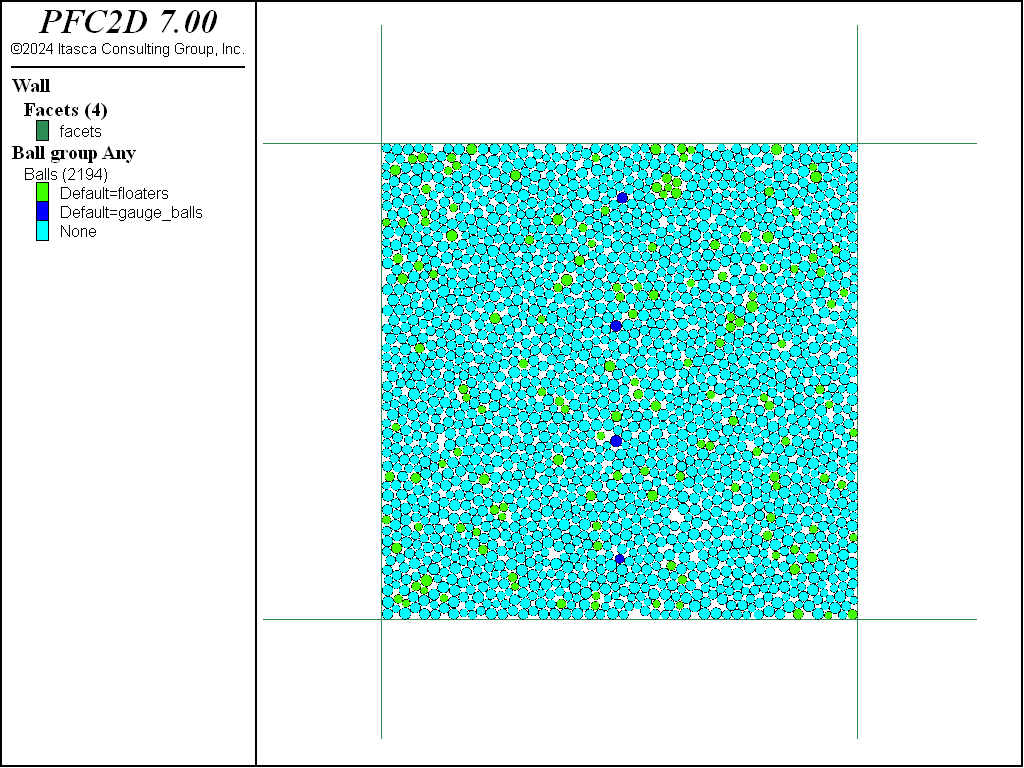
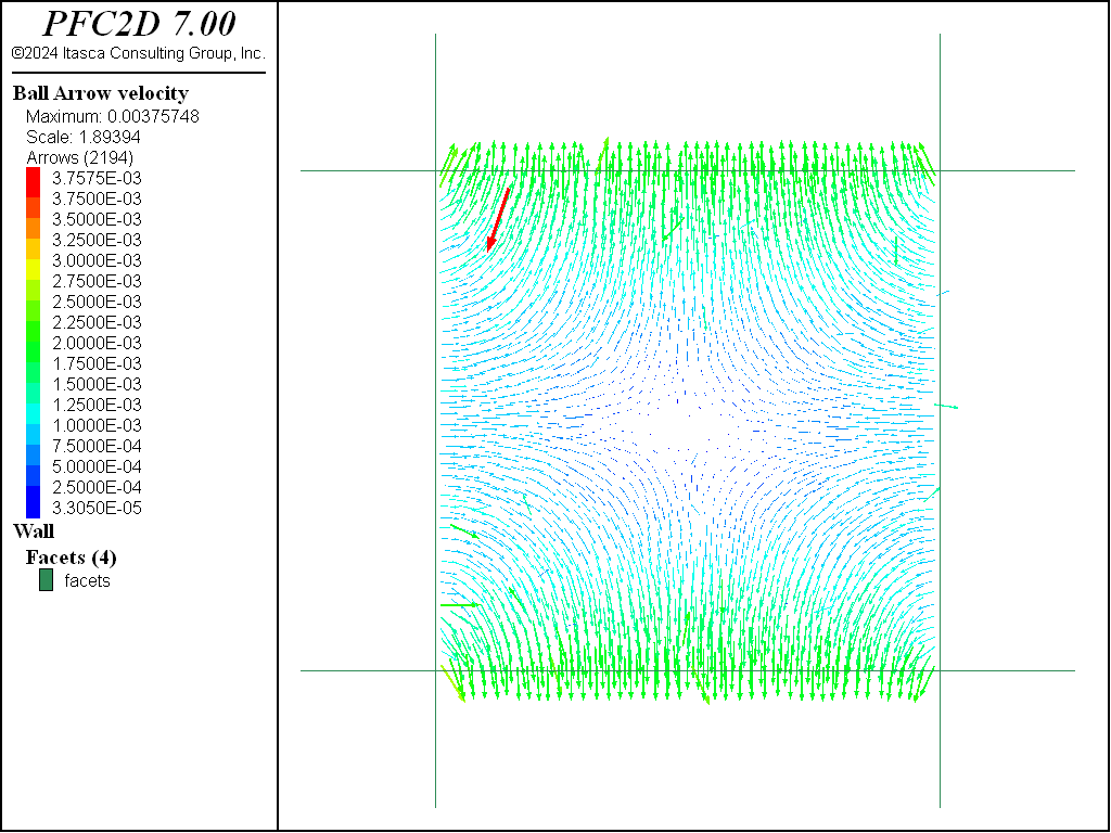
Figure 1 shows a loose specimen after gauge balls and floaters have been identified.

Figure 1: Loose assembly with balls colored by group identifiers.

Stress and Strain Measurement Utilities

Measuring Stress

Different approaches to measuring stress in a granular assembly are discussed below. The corresponding FISH functions are defined in the file “StressUtilities.p2fis”. Note that in PFC2D balls are assumed to be disks with unit thickness for stress calculations.

First, the reaction forces exerted by the specimen on the vessel walls can be used. The two functions below average the reaction forces on opposite walls, and divide them by the representative area of the walls in each direction to return the horizontal and vertical stress:

fish define wsxx
    global wp_left, wp_right, wly
    wsxx = 0.5*(wall.force.contact.x(wp_left) - ...
           wall.force.contact.x(wp_right))/ wly 
end

fish define wsyy
    global wp_bot, wp_top, wlx
    wsyy = 0.5*(wall.force.contact.y(wp_bot) -  ...
           wall.force.contact.y(wp_top)  )/ wlx
end

Alternatively, Measurement regions can be created within the model using the measure create command, and used to compute an average stress over contacts that lie in or intersect the measurement region (see here for details).

The same computation is defined in the “StressUtilities.p2fis” file (compute_spherestress function), providing a verification of the results computed by the measure logic.

fish define compute_spherestress(rad)
  command
    contact group 'insphere' remove
    contact group 'insphere' range circle radius [rad]
  endcommand
  global ssxx = 0.0
  global ssxy = 0.0
  global ssyx = 0.0
  global ssyy = 0.0
  loop foreach contact contact.groupmap("insphere","ball-ball")
    local cf = contact.force.global(contact)
    local cl = ball.pos(contact.end2(contact)) - ...
               ball.pos(contact.end1(contact))
    ssxx = ssxx + comp.x(cf) *comp.x(cl)
    ssxy = ssxy + comp.x(cf) *comp.y(cl)
    ssyx = ssyx + comp.y(cf) *comp.x(cl)
    ssyy = ssyy + comp.y(cf) *comp.y(cl)
  endloop
  local vol = (math.pi*rad^2)
  ssxx = - ssxx / vol
  ssxy = - ssxy / vol
  ssyx = - ssyx / vol
  ssyy = - ssyy / vol
end

This computation can be performed for a different probing volume (large enough compared to the particle sizes). For instance the function compute_averagestress in “StressUtilities.p2fis” computes the average stress over the entire vessel volume.

fish define compute_averagestress
  global asxx = 0.0
  global asxy = 0.0
  global asyx = 0.0
  global asyy = 0.0
  loop foreach local contact contact.list("ball-ball")
    local cforce =  contact.force.global(contact)
    local cl = ball.pos(contact.end2(contact)) - ...
               ball.pos(contact.end1(contact))
    asxx = asxx + comp.x(cforce)*comp.x(cl)
    asxy = asxy + comp.x(cforce)*comp.y(cl)
    asyx = asyx + comp.y(cforce)*comp.x(cl)
    asyy = asyy + comp.y(cforce)*comp.y(cl)
  endloop
  asxx = - asxx / (wlx*wly)
  asxy = - asxy / (wlx*wly)
  asyx = - asyx / (wlx*wly)
  asyy = - asyy / (wlx*wly)
end

The results that were obtained measuring the stress at the end of an isotropic consolidation stage to 500kPa confinement (see below) are listed in Table 1 for comparison. As expected, the compute_spherestress function returns the same values obtained using the Measure logic, as the operations are exactly the same and the stress is measured over the same region. Stresses computed by the compute_averagestress and compute_wallstress functions differ slightly due to the relatively small size of the specimen and different measurement techniques used, but remain within 3% of the target value.

Table 1: Stress Measurements - 2D Model

	Loose Specimen		Dense Specimen
	XX-Stress [Pa]	YY-Stress [Pa]	XX-Stress [Pa]	YY-Stress [Pa]
Measure Logic	-5.009178e+05	-4.932599e+05	-5.185070e+05	-5.147563e+05
compute_spherestress	-5.009178e+05	-4.932599e+05	-5.185070e+05	-5.147563e+05
compute_averagestress	-4.893537e+05	-4.890566e+05	-4.890899e+05	-4.888240e+05
compute_wallstress	-5.000043e+05	-4.999950e+05	-5.000057e+05	-4.999945e+05

Measuring Strain

Similar to stress, strain may be evaluated using several methods. Several approaches are discussed below, the corresponding FISH functions may be found in “StrainUtilities.p2fis”.

Macroscopic axial and lateral strains can also be computed from the relative displacement of the boundary walls as:

(1)\[\epsilon_{ii} = \frac{L_{ii} - L_{ii}^{(0)}}{L_{ii}^{(0)}}\]

where \(L_{ii}^{(0)}\) and \(L_{ii}\) are the initial and current length of the specimen in direction \(i\).

The Measure logic may be used to evaluate strain rate at a given step over a measurement region. Strain increments can therefore be accumulated at each iteration by using the computed value of the strain rate times the current timestep. Since the strain rate needs to be computed and strain increments accumulated during each cycle, this operation can be computationally intensive.

fish define ini_mstrain(sid)
  command
    ball attribute displacement multiply 0.0
  endcommand
  global mstrains = matrix(2,2)
  global mp = measure.find(sid)
end

fish define accumulate_mstrain
  global msrate =  measure.strain.rate(mp)
  global mstrains = mstrains + msrate * global.timestep
  global xxmstrain = mstrains(1,1)
  global xymstrain = mstrains(1,2)
  global yxmstrain = mstrains(2,1)
  global yymstrain = mstrains(2,2)
end

Another approach to evaluate strain relies on measuring relative displacements between gauge particles. This method has the advantage that both axial and tangential strain can be measured, but suffers from the discrete nature of the system. The function ini_gstrain in “StrainUtilities.p2fis” allows the placement of gauge particles for strain measurement. Four equally spaced gauge particles are identified along the \(y\)-axis using the ball.near FISH utility, and the group identifier gauge_balls is assigned. Their initial relative position is recorded, allowing for the computation of the strain in any moment, as shown in the xygstrain function for the computation of tangential strain.

fish define ini_gstrain(ly)
  local pos = vector(0.0,-0.5*ly)*0.75
  global gb1 = ball.near(pos)
  ball.group(gb1) = 'gauge_balls'
  pos = vector( 0.0,-0.5*ly)*0.25
  global gb2 = ball.near(pos)
  ball.group(gb2) = 'gauge_balls'
  pos = vector( 0.0, 0.5*ly)*0.25
  global gb3 = ball.near(pos)
  ball.group(gb3) = 'gauge_balls'
  pos = vector(0.0, 0.5*ly)*0.75
  global gb4 = ball.near(pos)
  ball.group(gb4) = 'gauge_balls'
  global gl12_0  = ball.pos(gb2) - ball.pos(gb1)
  global gl13_0  = ball.pos(gb3) - ball.pos(gb1)
  global gl14_0  = ball.pos(gb4) - ball.pos(gb1)
end

fish define xygstrain
  local gl12 = ball.pos(gb2) - ball.pos(gb1)
  global xygstrain12 = (comp.x(gl12) - comp.x(gl12_0))/ comp.y(gl12_0) 
  local gl13 = ball.pos(gb3) - ball.pos(gb1)
  global xygstrain13 =  (comp.x(gl13) - comp.x(gl13_0))/ comp.y(gl13_0) 
  local gl14 = ball.pos(gb4) - ball.pos(gb1)
  global xygstrain14 =  (comp.x(gl14) - comp.x(gl14_0))/ comp.y(gl14_0) 
  xygstrain = (xygstrain12 + xygstrain13 + xygstrain14) /3.0
end

Biaxial Test

The tools discussed in the previous sections are combined to perform a simple biaxial test. The biaxial test is performed in two stages: an isotropic consolidation stage during which the specimen is brought to equilibrium under a prescribed confining stress, followed by a biaxial compression in the vertical direction at constant lateral stress.

During the consolidation stage, the specimen is loaded in a strain-controlled fashion, but the velocities of the vessel boundary walls are adjusted using a servo-control mechanism so that a target confining stress is achieved.

During the biaxial compression stage, the servo-control is deactivated for the top and bottom walls that act as loading platens with constant velocity, but remains active for the left and right walls in order to maintain confinement. The stresses and strains experienced by the sample are determined in a macro fashion by computing the stress acting upon, and relative displacement of, opposite walls. The History logic is used to monitor the evolution of the system.

Servo-Control Mechanism

The wall servo command is used to set the activity status and parameters of the servo-control for each wall.

[txx = -5.0e5]
[tyy = -5.0e5]
wall servo activate on force-x [ txx*wly] ...
                       velocity-max 0.1 range set name 'vesselRight'
wall servo activate on force-x [-txx*wly] ...
                       velocity-max 0.1 range set name 'vesselLeft'
wall servo activate on force-y [ tyy*wlx] ...
                       velocity-max 0.1 range set name 'vesselTop'
wall servo activate on force-y [-tyy*wlx] ...
                       velocity-max 0.1 range set name 'vesselBottom'

Note that this command does take a force as input parameter, instead of a stress. THe reason is that the “active” area of a wall does depend on the model, and PFC has no information to evaluate it. For instance, in this model, the vessel walls have initially been expanded in order to accomodate motion during the tests, and the “active” sections of the walls correspond to the vessel dimensions wlx and wly. In order to apply a target stress, the force used as an inuput to the wall servo command must therefore be adjusted as wlx and wly evolve during the test. This is achieved by registering a function in the cycle sequence using the fish callback command (see this tutorial for a detailed discussion about callback functions).

fish define servo_walls
  wall.servo.force.x(wp_right) =   txx*wly
  wall.servo.force.x(wp_left)  =  -txx*wly
  wall.servo.force.y(wp_top)   =   tyy*wlx
  wall.servo.force.y(wp_bot)   =  -tyy*wlx
end
fish callback add servo_walls  9.0 

Isotropic Consolidation Stage

The file “CompactSpecimen.dat” is invoked to perform this stage. The initial dimensions of the vessel are computed, and the isotropic stress to be applied to the granular sample is defined. Both the vertical and horizontal walls move to gradually apply the required stress. The function servo_walls is registered to be executed before the resolution of the equation of motion during each cycle. Horizontal and vertical stresses are recorded during the simulation using the History logic. Orientation tracking is switched on (see the model orientation-tracking command) so that ball orientations can be tracked and visualized.

The model is cycled until the wall-based measured horizontal and vertical stresses are close to the prescribed stress (to a user-defined tolerance), and the average unbalanced force ratio, ratio-average, is less than or equal to 1e-6 (see the model solve ratio-average command). This complex stopping criterion is defined in the function stop_me, which is executed at the end of each cycle. It is registered as a solve limit with the model solve fish-halt command. The state of stress in each direction during the seating phase is depicted below.

[tol =  5e-3]
fish define stop_me
  if math.abs((wsyy - tyy)/tyy) > tol
    exit
  endif
  if math.abs((wsxx - txx)/txx) > tol
    exit
  endif
  if mech.solve("ratio-average") > 1e-6
    exit
  endif
  stop_me = 1
end

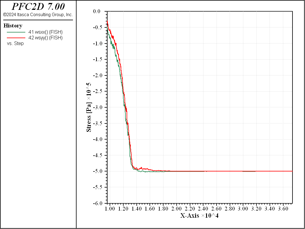
Figure 2: State of stress (computed from contact forces on boundary walls) at the end of the isotropic compression phase ( \(\sigma_{iso}\) = 1 MPa).

A measurement region is created to compute the porosity of the specimen at the end of this phase, and the alternate functions to compute stress discussed above are also invoked for comparison.

measure create id 1 rad [0.4*(math.min(lx0,ly0))]
[porosity = measure.porosity(measure.find(1))]
[compute_spherestress(0.4*(math.min(lx0,ly0)))]
[compute_averagestress]

The results listed in the table above compare the values of stress obtained with the different approaches for both the loose and dense specimen.

Deviatoric Loading Stage

The file “BiaxialTest.dat” is invoked to perform this stage.

Friction at ball-ball and ball-facet contacts, which was set to obtain the desired porosity of the specimen during the previous phases, is modified.

ball property 'fric' [ballFriction]
wall property 'fric' [wallFriction]

The equilibrated system is ready to be subjected to a biaxial test. An equal and opposite constant velocity is set to the upper and lower walls, performing a strain-controlled compression test. The velocity of the lateral walls is updated with the servo-control mechanism described previously to maintain the appropriate confining stress.

[rate = 0.2]
wall servo activate off range set name 'vesselTop' ...
                              set name 'vesselBottom' union 
wall attribute velocity-y [-rate*wly] range set name 'vesselTop'
wall attribute velocity-y [ rate*wly] range set name 'vesselBottom'

The initial dimensions of the vessel are computed, and the strain variables (axial, lateral, and volumetric strains) are set to zero. These values will be updated during the simulation as a function of the relative distance between the appropriate walls and recorded using the History logic.

[ly0 = wly]
[lx0 = wlx]
[wexx = 0.0]
[weyy = 0.0]
[wevol = 0.0]

fish define wexx
  wexx  = (wlx - lx0) / lx0 
end

fish define weyy
  weyy = (wly - ly0) / ly0
end

fish define wevol
  wevol = wexx + weyy
end

fish history name '51' wexx
fish history name '52' weyy
fish history name '53' wevol
history purge

The system is loaded to 7.5% vertical strain (see the target variable and its use in the stop_me function).

[stop_me = 0]
[target = 0.075]
fish define stop_me
  if weyy <= -target then
    stop_me = 1
  endif
end

Biaxial Tests on Dense and Loose Samples

The biaxial test is performed on a loose sample and on a dense sample in order to assess their differences. To generate either a loose or a dense granular packing, the appropriate value of friction at ball-ball contacts has been adjusted. The “Doall.dat” data file contains the commands to prepare a loose specimen, to compact it with a prescribed confining stress, and to finally perform a biaxial compression.

model new
;define ball and wall friction values to generate a loose sample
[ballFriction = 0.3 ]
[wallFriction = 0.0    ]
[filename = 'loose'    ]
program call 'MakeSpecimen'
model save ['specimen'+filename]
program call 'CompactSpecimen'
model save ['biaxial-iso'+filename]
program call 'BiaxialTest'
model save ['biaxial-final'+filename]

;---------BIAXIAL TEST ON A DENSE SAMPLE
model new
;define ball and wall friction values to generate a dense sample
[ballFriction = 0.0 ]
[wallFriction = 0.0    ]
[filename = 'dense'  ]
program call 'MakeSpecimen'
model save ['specimen'+filename]
program call 'CompactSpecimen'
model save ['biaxial-iso'+filename]
[ballFriction = 0.3  ]
program call 'BiaxialTest'
model save ['biaxial-final'+filename]

To obtain a loose specimen, a friction coefficient of 0.3 is used for ball-ball contacts. This value is maintained during the entire simulation (preparation of the specimen, isotropic compaction, biaxial compression). Wall friction is set to zero so that shear forces won’t develop in ball-facet contacts. The use of frictionless walls reduces boundary effects during the preparation and compression phases.

To prepare a dense specimen, the friction at ball-ball contacts is initially set to zero. After the preparation and compaction phases, but prior to the biaxial compression, the friction coefficient for ball-ball contacts is set to the desired value of 0.3.

A porosity of \(n\) = 0.187 and \(n\) = 0.151 is measured at the end of the consolidation stage for the loose and dense specimen, respectively.

As can be observed from the stress-strain curves of Figures 3 and 4, the typical behavior of granular materials during a biaxial test is recovered. A marked peak characterizes the stress-strain curve for the dense sample, while the loose specimen evolves monotically to the same critical state. In terms of volumetric deformation, the loose specimen undergoes contraction, while the dense specimen shows a transition from contraction to dilation.

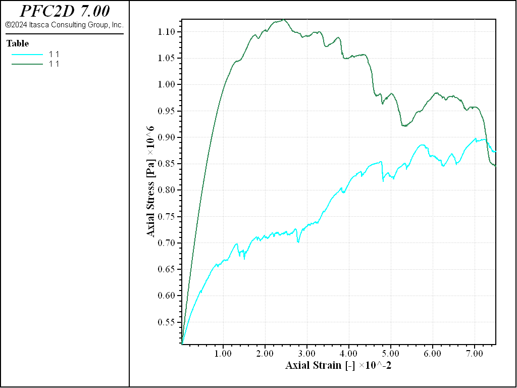
Figure 3: Stress vs. strain curves for loose (blue) and dense (red) specimen subjected to biaxial compression.

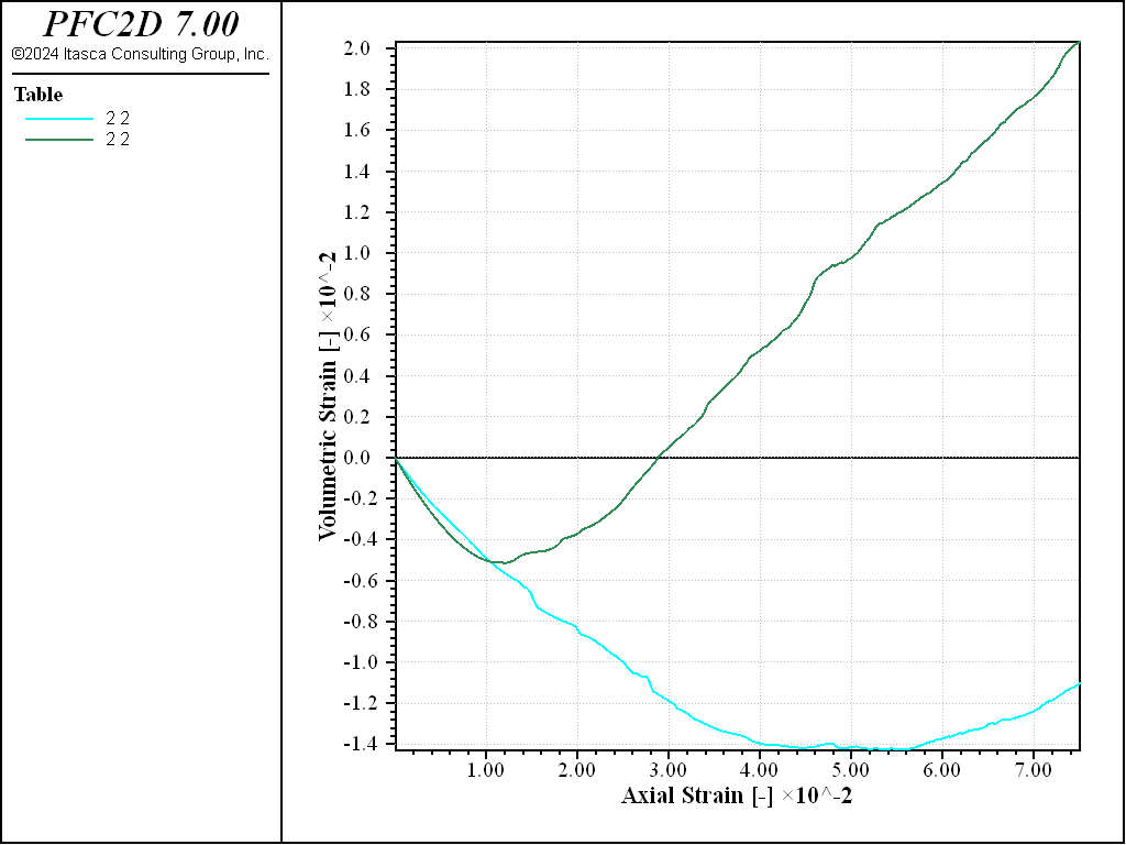
Figure 4: Volumetric strain evolution for loose (blue) and dense(red) specimen subjected to biaxial compression.

Computation of Elastic Parameters

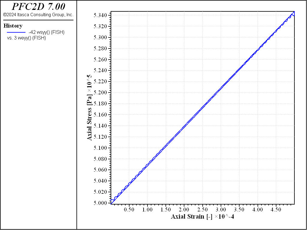
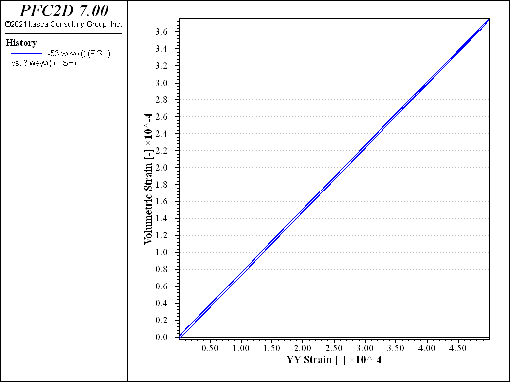
The material elastic properties can be determined by performing a loading/unloading test under elastic conditions, measuring the Young’s modulus and Poisson’s ratio. The procedure is implemented in the “LoadUnload.dat” file. Plots of axial deviatoric stress and volumetric strain versus axial strain are shown for the dense specimen in Figures 5 and 6. From these plots, the Young’s modulus is

(2)\[E = \frac{\Delta \sigma_a}{\Delta \varepsilon_a} \simeq 70 \mbox{MPa}\]

and the Poisson’s ratio is

(3)\[\nu = \frac{\Delta \varepsilon_r}{\Delta \varepsilon_a} \simeq 0.2\]

The shear modulus can be estimated using the expression

(4)\[G = \frac{E}{2(1+\nu)} \simeq 30 \mbox{MPa}\]

Figure 5: Axial deviatoric stress vs. axial strain for elastic load/unload test (dense sample).

Figure 6: Volumetric strain vs. axial strain for elastic load/unload test (dense sample).

Simple Shear and Pure Shear Tests

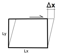
In this section, the preparation of a shear test to be performed on the compacted sample is presented. The dense sample is used for the shear simulations. A simple shear test and a pure shear test are performed (see Figures 7 and 8).

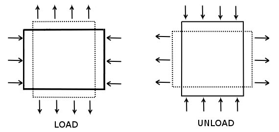
Simple shear (Figure 7) is a special case of deformation where only one component of velocity vector has a nonzero value. In solid mechanics, it is defined as an isochoric plane deformation in which there is a set of line elements with given reference orientations that do not change length and orientation during the deformation. The shear strain is defined in this case as

(5)\[\gamma_{xy} = \frac{\Delta x}{L_y}\]

where \(L_y\) denotes the length along the y direction.

Figure 7: Boundary conditions for a simple shear test.

Pure shear (Figure 8) is an example of irrotational strain in which a body is elongated in one direction while being shortened perpendicularly. Pure shear stress, \(\tau\), is related to pure shear strain, \(\gamma\), by the following equation:

(6)\[\tau = \gamma G\]

where \(G\) is the shear modulus. Under these conditions, the shear strain can be computed as

(7)\[\gamma_{xy} = \frac{\Delta x}{L_y} + \frac{\Delta y}{L_x}\]

Figure 8: Boundary conditions for a pure shear test.

Simple Shear Test

The data file “Doall.dat” contains the commands to restore the compacted dense sample, define the friction coefficients for ball-ball and ball-facet contacts, and to launch the simple shear test. Note that friction is introduced at ball-facet contacts to ensure a homogeneous response of the specimen.

[filename = 'dense']
model restore ['biaxial-iso'+filename]
[ballFriction = 0.3  ]
[wallFriction = 0.3  ]
program call 'SimpleShear'
model save 'simpleshear-final'

Select lines of the data file “SimpleShear.dat” are described below. First operation, the servo-mechanism is deactivated for all walls, and frictional properties are updated.

model large-strain on
wall servo activate off
fish callback remove servo_walls 1.0 

;define ball and wall friction property
ball property 'fric' [ballFriction]
wall property 'fric' [wallFriction]

A translational velocity is assigned to the top wall, while a rotational velocity is specified for the lateral walls.

[rate = 1.0]
wall attribute velocity-x [ 1.0*rate*wly] range set name 'vesselTop'
wall attribute rotation-center [-0.5*wlx] [-0.5*wly] ...
               spin [-1.0*rate] range set name 'vesselLeft'
wall attribute rotation-center [0.5*wlx] [-0.5*wly] ...
               spin [-1.0*rate] range set name 'vesselRight'

Average shear stress (see “StressUtilities.p2fis” utility file) and average shear strain (using eq. (5)) are computed.

As described in the previous sections, the increments of strain can be computed at each timestep using the value of strain rate measured within a measurement region. The stress can also be accessed via the measure region. Note the use of the fish callback command to call the function that computes the strain during each cycle. Notably, the FISH function is called after the equations of motion of the system are solved. The cycle numbers associated with each cycle operation can be listed with the program list cycle-sequence command.

All the strain and stress-related quantities are stored using the fish history command.

[defxy = 0]
fish define shear_strain
  defxy = defxy + rate*global.timestep
end

[ini_mstrain(1)]

fish history name '11' xxmstrain
fish history name '12' xymstrain
fish history name '13' yxmstrain
fish history name '14' yymstrain

measure history name '31' stress-xx id 1 
measure history name '32' stress-xy id 1 
measure history name '33' stress-yx id 1 
measure history name '34' stress-yy id 1

fish history name '61' asxy
fish history name '51' defxy

[ini_gstrain(wly)]
fish history name '21' xygstrain
fish history name '22' xygstrain12
fish history name '23' xygstrain13
fish history name '24' xygstrain14

fish callback add shear_strain          2.0 
fish callback add accumulate_mstrain    11.0 
fish callback add compute_averagestress 43.0 

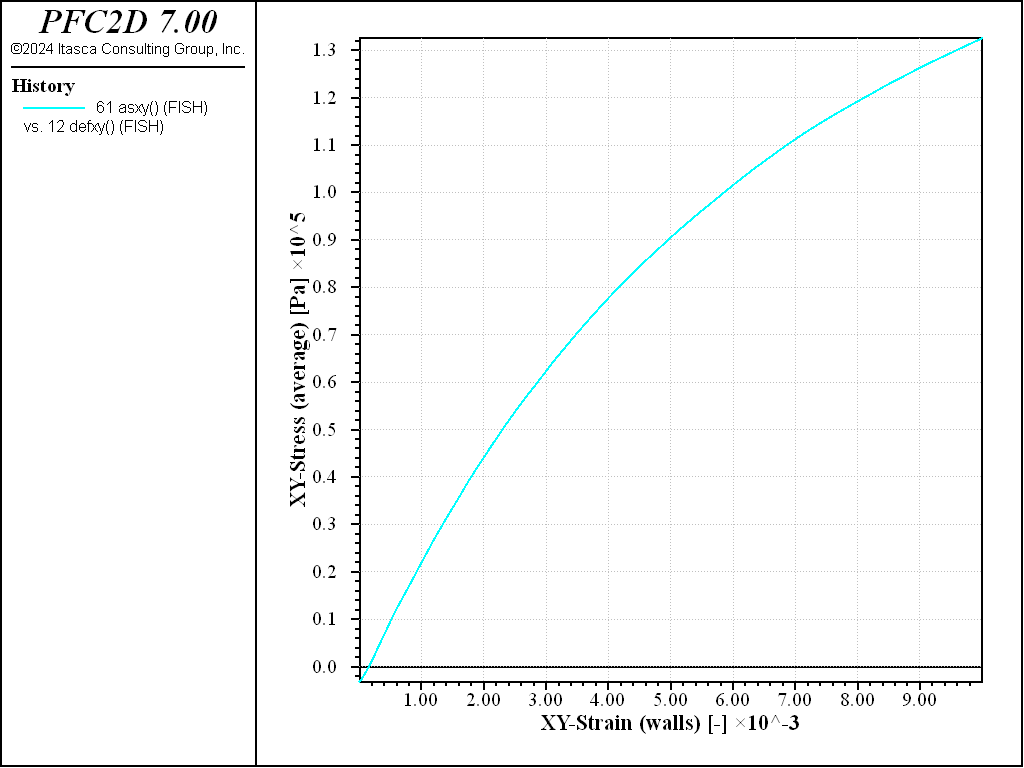
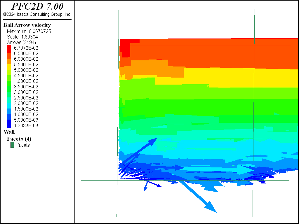
Figures 9 and 10 show the shear stress versus strain as measured by the Measure logic, or by computing an average over the whole specimen. Both techniques to measure stress and strain are valid. The material response is shown in Figure 11.

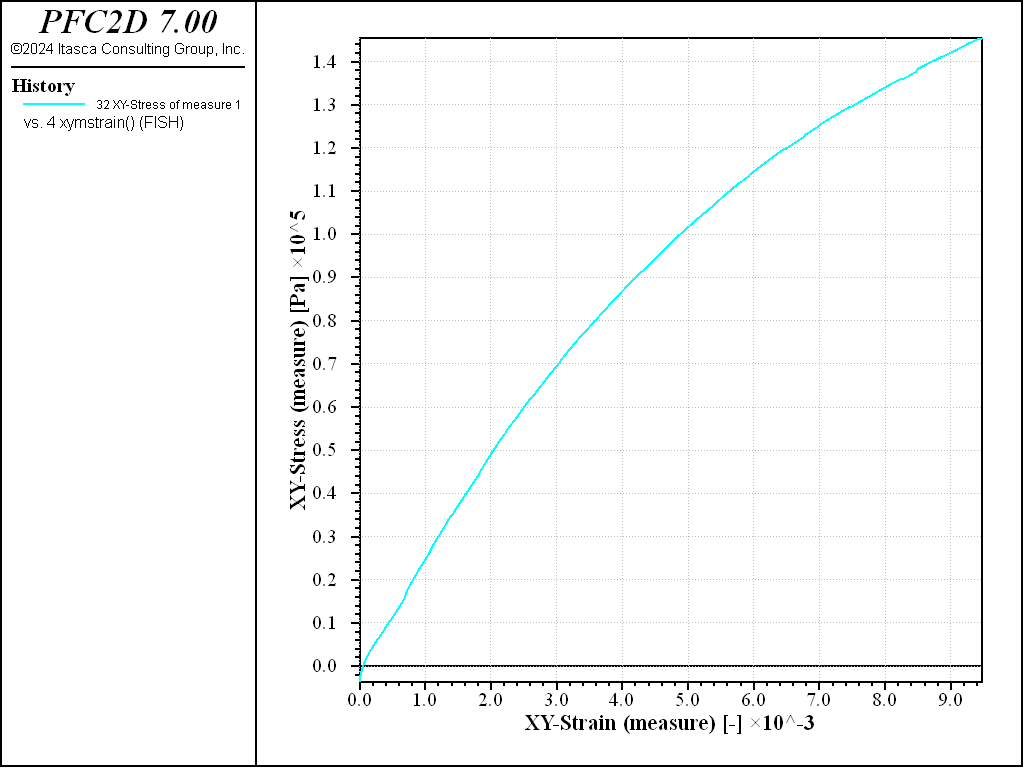
Figure 9: Simple shear test on a dense sample. Stress-strain curve (data obtained using the measure logic).

Figure 10: Simple shear test on a dense sample. Stress-strain curve (average values).

Figure 11: Simple shear test on a dense sample. Ball and wall velocities.

Pure Shear Test

The data file “Doall.dat” contains the commands used to restore the compacted dense sample, define the friction property of ball-ball and ball-facet contacts, and launch the pure shear test.

[filename = 'dense']
model restore ['biaxial-iso'+filename]
[ballFriction = 0.3  ]
[wallFriction = 0.3  ]
program call 'PureShear'
model save 'pureshear-final'

The file “PureShear.dat” is invoked to perform the calculation. In this file, the servo-mechanism is deactivated for all walls and appropriate frictional properties are assigned. The initial dimensions of the vessel are stored to compute the shear deformation during the simulation using eq. (7), and tangential stress is computed using the following expression:

(8)\[\tau_{xy} = \frac{\sigma_1 - \sigma_2}{2} = \frac{\sigma_h - \sigma_v}{2}\]

wall servo activate off
fish callback remove servo_walls 1.0 

;define ball and wall friction property
ball property 'fric' [ballFriction]
wall property 'fric' [wallFriction]

[ly0 = wly]
[lx0 = wlx]

[defxy = 0]
[tauxy = 0]
fish define shear_strain_stress
  x_strain = (wlx-lx0)
  y_strain = (wly-ly0)
  defxy = x_strain/ly0 + y_strain/lx0
  tauxy = (wsxx-wsyy)/2
end

Load/unload cycles are performed by registering the function cyclic_shear in the cycle sequence.

[load = 1]
[rate = 0.001]
[xfactor = 0.0]
[yfactor = 0.0]
fish define cyclic_shear
  wall.vel.x(wp_left)  =        xfactor*rate ; left wall
  wall.vel.x(wp_right) = -1.0 * xfactor*rate ; right wall
  wall.vel.y(wp_top)   = -1.0 * yfactor*rate ; top wall
  wall.vel.y(wp_bot)   =        yfactor*rate ; bottom wall
  if defxy < 0.0005
    if load = 1
      xfactor = 1.0
      yfactor = -2.0
      exit
    else
      if defxy < -0.0005
        load = 1
        exit
      endif
      exit
    endif
  else
    xfactor = -1.0
    yfactor = 2.0
    load = 0
  endif
end

The fish callback command is used to execute this function during each cycle, together with the functions that compute the shear stress and strain.

fish callback add shear_strain_stress 2.0 
fish callback add cyclic_shear        3.0 

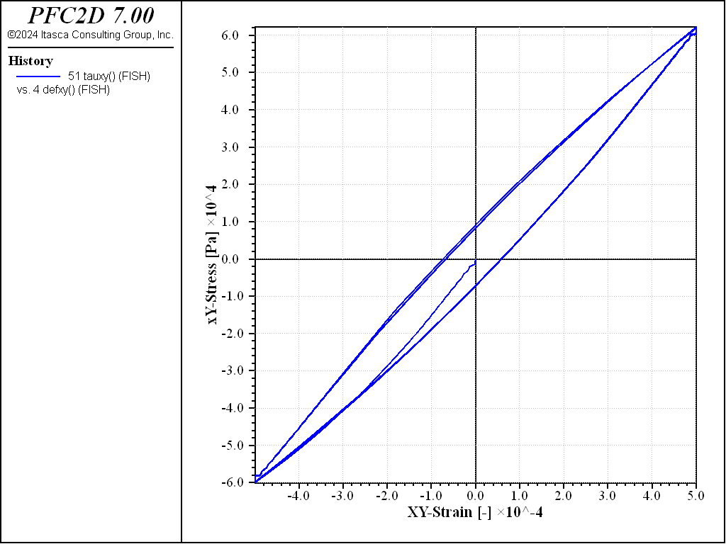
Figure 12 shows the evolution of shear stress and strain during the simulation. The curve shows a hysteresis effect. Using eq. (6), the shear modulus can be estimated, obtaining \(G \simeq 100 \mbox{MPa}\).

Figure 12: Pure shear test on a dense sample. Stress-strain curve.

Figure 13: Pure shear test on a dense sample. Ball velocities.

Discussion

This example demonstrates genesis and testing of loose and dense granular specimen in 2D, and discusses different approaches that can be used to probe the mechanical response of the models. The same approach can be used in 3D, and for bonded-particle models. The material genesis stage remains simple in this example. For applied models, care should be taken in order to reproduce a microstructure that is representative of the material being investigated.

Data Files

StrainUtilities.p2fis

; excerpt-mxlr-start
fish define ini_mstrain(sid)
  command
    ball attribute displacement multiply 0.0
  endcommand
  global mstrains = matrix(2,2)
  global mp = measure.find(sid)
end

fish define accumulate_mstrain
  global msrate =  measure.strain.rate(mp)
  global mstrains = mstrains + msrate * global.timestep
  global xxmstrain = mstrains(1,1)
  global xymstrain = mstrains(1,2)
  global yxmstrain = mstrains(2,1)
  global yymstrain = mstrains(2,2)
end
; excerpt-mxlr-end

; excerpt-ybnr-start
fish define ini_gstrain(ly)
  local pos = vector(0.0,-0.5*ly)*0.75
  global gb1 = ball.near(pos)
  ball.group(gb1) = 'gauge_balls'
  pos = vector( 0.0,-0.5*ly)*0.25
  global gb2 = ball.near(pos)
  ball.group(gb2) = 'gauge_balls'
  pos = vector( 0.0, 0.5*ly)*0.25
  global gb3 = ball.near(pos)
  ball.group(gb3) = 'gauge_balls'
  pos = vector(0.0, 0.5*ly)*0.75
  global gb4 = ball.near(pos)
  ball.group(gb4) = 'gauge_balls'
  global gl12_0  = ball.pos(gb2) - ball.pos(gb1)
  global gl13_0  = ball.pos(gb3) - ball.pos(gb1)
  global gl14_0  = ball.pos(gb4) - ball.pos(gb1)
end

fish define xygstrain
  local gl12 = ball.pos(gb2) - ball.pos(gb1)
  global xygstrain12 = (comp.x(gl12) - comp.x(gl12_0))/ comp.y(gl12_0) 
  local gl13 = ball.pos(gb3) - ball.pos(gb1)
  global xygstrain13 =  (comp.x(gl13) - comp.x(gl13_0))/ comp.y(gl13_0) 
  local gl14 = ball.pos(gb4) - ball.pos(gb1)
  global xygstrain14 =  (comp.x(gl14) - comp.x(gl14_0))/ comp.y(gl14_0) 
  xygstrain = (xygstrain12 + xygstrain13 + xygstrain14) /3.0
end
; excerpt-ybnr-end

StressUtilities.p2fis

; excerpt-rxlr-start
fish define wsxx
    global wp_left, wp_right, wly
    wsxx = 0.5*(wall.force.contact.x(wp_left) - ...
           wall.force.contact.x(wp_right))/ wly 
end

fish define wsyy
    global wp_bot, wp_top, wlx
    wsyy = 0.5*(wall.force.contact.y(wp_bot) -  ...
           wall.force.contact.y(wp_top)  )/ wlx
end
; excerpt-rxlr-end

; excerpt-xmps-start
fish define compute_averagestress
  global asxx = 0.0
  global asxy = 0.0
  global asyx = 0.0
  global asyy = 0.0
  loop foreach local contact contact.list("ball-ball")
    local cforce =  contact.force.global(contact)
    local cl = ball.pos(contact.end2(contact)) - ...
               ball.pos(contact.end1(contact))
    asxx = asxx + comp.x(cforce)*comp.x(cl)
    asxy = asxy + comp.x(cforce)*comp.y(cl)
    asyx = asyx + comp.y(cforce)*comp.x(cl)
    asyy = asyy + comp.y(cforce)*comp.y(cl)
  endloop
  asxx = - asxx / (wlx*wly)
  asxy = - asxy / (wlx*wly)
  asyx = - asyx / (wlx*wly)
  asyy = - asyy / (wlx*wly)
end
; excerpt-xmps-end

; excerpt-womr-start
fish define compute_spherestress(rad)
  command
    contact group 'insphere' remove
    contact group 'insphere' range circle radius [rad]
  endcommand
  global ssxx = 0.0
  global ssxy = 0.0
  global ssyx = 0.0
  global ssyy = 0.0
  loop foreach contact contact.groupmap("insphere","ball-ball")
    local cf = contact.force.global(contact)
    local cl = ball.pos(contact.end2(contact)) - ...
               ball.pos(contact.end1(contact))
    ssxx = ssxx + comp.x(cf) *comp.x(cl)
    ssxy = ssxy + comp.x(cf) *comp.y(cl)
    ssyx = ssyx + comp.y(cf) *comp.x(cl)
    ssyy = ssyy + comp.y(cf) *comp.y(cl)
  endloop
  local vol = (math.pi*rad^2)
  ssxx = - ssxx / vol
  ssxy = - ssxy / vol
  ssyx = - ssyx / vol
  ssyy = - ssyy / vol
end
; excerpt-womr-end

MakeSpecimen.dat

model large-strain on
; fname: make_specimen.p2dat
;
; Generate a dense granular assembly within a box
;
; ========================================================================

; Load utility FISH functions for later use
; excerpt-slng-start
program call 'StrainUtilities.p2fis' suppress  
program call 'StressUtilities.p2fis' suppress
; excerpt-slng-end

; Define domain extent and default contact model and properties in the CMAT
; note that since friction is not set (and defaults to zero), shear forces
; won't develop
; excerpt-aobs-start
model domain extent -0.1 0.1 
contact cmat default model linear method deformability emod 1.0e8 kratio 2.5
; excerpt-aobs-end

; Generate a box-wall comprised of 4 independant walls. Each wall is expanded 
; in preparation for upcoming motion, and global FISH variables that hold 
; pointers to the walls are created for convenience. 
; excerpt-inal-start
wall generate name 'vessel' box -0.035 0.035 expand 1.5
[wp_left  = wall.find('vesselLeft')]
[wp_right = wall.find('vesselRight')]
[wp_bot   = wall.find('vesselBottom')]
[wp_top   = wall.find('vesselTop')]
; excerpt-inal-end

; FISH functions to get vessel dimensions
; excerpt-zpmw-start
fish define wlx
  wlx  = wall.pos.x(wp_right) - wall.pos.x(wp_left)
end
fish define wly
  wly  = wall.pos.y(wp_top)   - wall.pos.y(wp_bot)
end
; excerpt-zpmw-end

; Generate a cloud of overlapping balls with a target porosity
; and assign density and local damping attributes
; excerpt-qoxf-start
model random 10001
ball distribute porosity 0.2 radius 0.0006 0.0009 box -0.035 0.035
; excerpt-qoxf-end
ball attribute density 2500.0 damp 0.7
;define ball and wall friction property
; excerpt-wing-start
ball property 'fric' [ballFriction]
wall property 'fric' [wallFriction]
; excerpt-wing-end
; solve to equilibr'ium
; excerpt-unlw-start
model cycle 1000 calm 10
model solve ratio-average 1e-5
model calm
; excerpt-unlw-end

; identify floaters using FISH function defined in make_utilities.p2fis
; excerpt-enxe-start
fish define identify_floaters
  loop foreach local ball ball.list
    ball.group.remove(ball,'floaters')
    local contactmap = ball.contactmap(ball)
    local size = map.size(contactmap)
    if size <= 1 then
      ball.group(ball) = 'floaters'
    endif
  endloop
end
[identify_floaters]
[ini_gstrain(wly)]
; excerpt-enxe-end

program return
; ========================================================================
; eof: make_specimen.p2dat

CompactSpecimen.dat

model large-strain on
[ly0 = wly]
[lx0 = wlx]
[v0 = wlx*wly]

; excerpt-ionr-start
[txx = -5.0e5]
[tyy = -5.0e5]
wall servo activate on force-x [ txx*wly] ...
                       velocity-max 0.1 range set name 'vesselRight'
wall servo activate on force-x [-txx*wly] ...
                       velocity-max 0.1 range set name 'vesselLeft'
wall servo activate on force-y [ tyy*wlx] ...
                       velocity-max 0.1 range set name 'vesselTop'
wall servo activate on force-y [-tyy*wlx] ...
                       velocity-max 0.1 range set name 'vesselBottom'
; excerpt-ionr-end

; excerpt-vvre-start
fish define servo_walls
  wall.servo.force.x(wp_right) =   txx*wly
  wall.servo.force.x(wp_left)  =  -txx*wly
  wall.servo.force.y(wp_top)   =   tyy*wlx
  wall.servo.force.y(wp_bot)   =  -tyy*wlx
end
fish callback add servo_walls  9.0 
; excerpt-vvre-end

fish history name '41' wsxx
fish history name '42' wsyy 

model orientation-tracking on
model calm

; excerpt-plnm-start
[tol =  5e-3]
fish define stop_me
  if math.abs((wsyy - tyy)/tyy) > tol
    exit
  endif
  if math.abs((wsxx - txx)/txx) > tol
    exit
  endif
  if mech.solve("ratio-average") > 1e-6
    exit
  endif
  stop_me = 1
end
; excerpt-plnm-end

ball attribute displacement multiply 0.0
model solve fish-halt stop_me

; excerpt-aaar-start
measure create id 1 rad [0.4*(math.min(lx0,ly0))]
[porosity = measure.porosity(measure.find(1))]
[compute_spherestress(0.4*(math.min(lx0,ly0)))]
[compute_averagestress]
; excerpt-aaar-end

[identify_floaters]

program return

LoadUnload.dat

model large-strain on
;define ball and wall friction property
ball property 'fric' [ballFriction]
wall property 'fric' [wallFriction]

[rate = 0.01]
wall attribute velocity-y [-rate*wly] range set name 'vesselTop'
wall attribute velocity-y [ rate*wly] range set name 'vesselBottom'
wall servo activate off range set name 'vesselTop' ...
                              set name 'vesselBottom' union 
model calm

[ly0 = wly]
[lx0 = wlx]
[wsyy0 = wsyy]

[wexx = 0.0]
[weyy = 0.0]
[wevol = 0.0]
fish define wexx
  wexx  = 2.0*(wlx - lx0) / (wlx+lx0) 
end

fish define weyy
  weyy = 2.0*(wly - ly0) / (wly+ly0)
end

fish define wevol
  wevol = wexx + weyy
end

fish history name '51' weyy
fish history name '52' wexx
fish history name '53' wevol
history purge

[stop_load = 0]
[target = 5e-4]
fish define stop_load
  if -weyy >= target then
    stop_load = 1
  endif
end
model solve fish-halt stop_load

[young_modulus = (wsyy-wsyy0)/weyy]
[poisson_ratio = -wexx/weyy]
[shear_modulus = 0.5*young_modulus/(1+poisson_ratio)]

model save 'biaxial-load'

wall attribute velocity-y [ rate*wly] range set name 'vesselTop'
wall attribute velocity-y [-rate*wly] range set name 'vesselBottom'

[stop_unload = 0]
fish define stop_unload
  if weyy >= 0.0 then
    stop_unload = 1
  endif
end
model solve fish-halt stop_unload

BiaxialTest.dat

model large-strain on
;define ball and wall friction property
; excerpt-esar-start
ball property 'fric' [ballFriction]
wall property 'fric' [wallFriction]
; excerpt-esar-end

; excerpt-oncc-start
[ly0 = wly]
[lx0 = wlx]
[wexx = 0.0]
[weyy = 0.0]
[wevol = 0.0]

fish define wexx
  wexx  = (wlx - lx0) / lx0 
end

fish define weyy
  weyy = (wly - ly0) / ly0
end

fish define wevol
  wevol = wexx + weyy
end

fish history name '51' wexx
fish history name '52' weyy
fish history name '53' wevol
history purge
; excerpt-oncc-end

; excerpt-inrw-start
[rate = 0.2]
wall servo activate off range set name 'vesselTop' ...
                              set name 'vesselBottom' union 
wall attribute velocity-y [-rate*wly] range set name 'vesselTop'
wall attribute velocity-y [ rate*wly] range set name 'vesselBottom'
; excerpt-inrw-end
; excerpt-prlr-start
[stop_me = 0]
[target = 0.075]
fish define stop_me
  if weyy <= -target then
    stop_me = 1
  endif
end
; excerpt-prlr-end

ball attribute displacement multiply 0.0
model calm
model solve fish-halt stop_me

program return

MeasureStress.dat

;restore specimen

;measure create id 1 radius [0.4*math.min(wlx,wly)]
;list measure

;set echo off
;  program call 004_stress_utilities.p2fis
;set echo on

[compute_averagestress]
;[compute_wallstress]
[compute_spherestress([0.3*math.min(wlx,wly)])]

program return

PureShear.dat

model large-strain on
; excerpt-ttnr-start
wall servo activate off
fish callback remove servo_walls 1.0 

;define ball and wall friction property
ball property 'fric' [ballFriction]
wall property 'fric' [wallFriction]

[ly0 = wly]
[lx0 = wlx]

[defxy = 0]
[tauxy = 0]
fish define shear_strain_stress
  x_strain = (wlx-lx0)
  y_strain = (wly-ly0)
  defxy = x_strain/ly0 + y_strain/lx0
  tauxy = (wsxx-wsyy)/2
end
; excerpt-ttnr-end

; excerpt-ioxx-start
[load = 1]
[rate = 0.001]
[xfactor = 0.0]
[yfactor = 0.0]
fish define cyclic_shear
  wall.vel.x(wp_left)  =        xfactor*rate ; left wall
  wall.vel.x(wp_right) = -1.0 * xfactor*rate ; right wall
  wall.vel.y(wp_top)   = -1.0 * yfactor*rate ; top wall
  wall.vel.y(wp_bot)   =        yfactor*rate ; bottom wall
  if defxy < 0.0005
    if load = 1
      xfactor = 1.0
      yfactor = -2.0
      exit
    else
      if defxy < -0.0005
        load = 1
        exit
      endif
      exit
    endif
  else
    xfactor = -1.0
    yfactor = 2.0
    load = 0
  endif
end
; excerpt-ioxx-end

fish history name '51' tauxy
fish history name '61' defxy

; excerpt-nnvv-start
fish callback add shear_strain_stress 2.0 
fish callback add cyclic_shear        3.0 
; excerpt-nnvv-end

model orientation-tracking on
model solve time 0.2

SimpleShear.dat

; excerpt-oppo-start
model large-strain on
wall servo activate off
fish callback remove servo_walls 1.0 

;define ball and wall friction property
ball property 'fric' [ballFriction]
wall property 'fric' [wallFriction]
; excerpt-oppo-end

; excerpt-ubvy-start
[rate = 1.0]
wall attribute velocity-x [ 1.0*rate*wly] range set name 'vesselTop'
wall attribute rotation-center [-0.5*wlx] [-0.5*wly] ...
               spin [-1.0*rate] range set name 'vesselLeft'
wall attribute rotation-center [0.5*wlx] [-0.5*wly] ...
               spin [-1.0*rate] range set name 'vesselRight'
; excerpt-ubvy-end

; excerpt-qzzz-start
[defxy = 0]
fish define shear_strain
  defxy = defxy + rate*global.timestep
end

[ini_mstrain(1)]

fish history name '11' xxmstrain
fish history name '12' xymstrain
fish history name '13' yxmstrain
fish history name '14' yymstrain

measure history name '31' stress-xx id 1 
measure history name '32' stress-xy id 1 
measure history name '33' stress-yx id 1 
measure history name '34' stress-yy id 1

fish history name '61' asxy
fish history name '51' defxy

[ini_gstrain(wly)]
fish history name '21' xygstrain
fish history name '22' xygstrain12
fish history name '23' xygstrain13
fish history name '24' xygstrain14

fish callback add shear_strain          2.0 
fish callback add accumulate_mstrain    11.0 
fish callback add compute_averagestress 43.0 
; excerpt-qzzz-end

model orientation-tracking on
model solve time 0.01

Doall.dat

;---------BIAXIAL TEST ON A LOOSE SAMPLE
; excerpt-nror-start
model new
;define ball and wall friction values to generate a loose sample
[ballFriction = 0.3 ]
[wallFriction = 0.0    ]
[filename = 'loose'    ]
program call 'MakeSpecimen'
model save ['specimen'+filename]
program call 'CompactSpecimen'
model save ['biaxial-iso'+filename]
program call 'BiaxialTest'
model save ['biaxial-final'+filename]

;---------BIAXIAL TEST ON A DENSE SAMPLE
model new
;define ball and wall friction values to generate a dense sample
[ballFriction = 0.0 ]
[wallFriction = 0.0    ]
[filename = 'dense'  ]
program call 'MakeSpecimen'
model save ['specimen'+filename]
program call 'CompactSpecimen'
model save ['biaxial-iso'+filename]
[ballFriction = 0.3  ]
program call 'BiaxialTest'
model save ['biaxial-final'+filename]
; excerpt-nror-end

;---------ESTIMATION OF ELASTIC PARAMETERS - LOAD UNLOAD TEST
[filename = 'dense']
model restore ['biaxial-iso'+filename]
[ballFriction = 0.3  ]
program call 'LoadUnload'
model save 'biaxial-unload'

;---------SIMPLE SHEAR TEST ON A DENSE SAMPLE
; excerpt-nnaa-start
[filename = 'dense']
model restore ['biaxial-iso'+filename]
[ballFriction = 0.3  ]
[wallFriction = 0.3  ]
program call 'SimpleShear'
model save 'simpleshear-final'
; excerpt-nnaa-end

;---------PURE SHEAR TEST ON A DENSE SAMPLE
; excerpt-ewwa-start
[filename = 'dense']
model restore ['biaxial-iso'+filename]
[ballFriction = 0.3  ]
[wallFriction = 0.3  ]
program call 'PureShear'
model save 'pureshear-final'
; excerpt-ewwa-end

program return

Endnotes

[1]	To view this project in PFC, use the program menu. Help ▼ Examples…   ⮡   PFC     ⮡   Examples       ⮡   Granular         ⮡   Granular.prj