Examples • Verification Problems

Simply Supported Orthotropic Plate

Problem Statement

Note

The project file for this example is available to be viewed/run in FLAC3D.[1] The main data files used are shown at the end of this example. The remaining data files can be found in the project.

The deflection and stress are determined numerically for the case of a simply supported rectangular orthotropic plate subjected to a uniformly distributed load.

Closed-Form Solution

The analytic solution for this problem is given by Ugural (1981, pp. 144-145). Consider a rectangular plate of sides \(a\) and \(b\), simply supported on all edges, subjected to a uniformly distributed load, \(p_0\), and with principal directions of orthotropy aligned with the \(x\)- and \(y\)-axes as shown in Figure 1.

Figure 1: Rectangular plate and coordinate system used to express the closed-form solution.

The deflection (\(w\)) bending stress resultants (\(M_x\), \(M_y\), and \(M_{xy}\)) and transverse-shear stress resultants (\(Q_x\) and \(Q_y\)) are given by

\[w = {{16 p_0} \over {\pi^6}} \sum^{\infty}_m \sum^{\infty}_n \Biggl[{1 \over \beta}\Biggr] {\rm sin} (m \pi x / a) {\rm sin} (n \pi y / b)\]

\[M_x = {{16 p_0} \over {\pi^4}} \sum^{\infty}_m \sum^{\infty}_n \Biggl[{{D_x (m^2 / a^2) + D_{xy} (n^2 / b^2)} \over {\beta}}\Biggr] {\rm sin} (m \pi x / a) {\rm sin} (n \pi y / b)\]

\[M_y = {{16 p_0} \over {\pi^4}} \sum^{\infty}_m \sum^{\infty}_n \Biggl[{{D_{xy} (m^2 / a^2) + D_y (n^2 / b^2)} \over {\beta}}\Biggr] {\rm sin} (m \pi x / a) {\rm sin} (n \pi y / b)\]

\[M_{xy} = {{16 p_0} \over {\pi^4}} \sum^{\infty}_m \sum^{\infty}_n \Biggl[{{2G_{xy} (mn/ab)} \over {\beta}}\Biggr] {\rm cos} (m \pi x / a) {\rm cos} (n \pi y / b)\]

\[Q_x = {{16 p_0} \over {\pi^4}} \sum^{\infty}_m \sum^{\infty}_n \Biggl[{{D_x (m^3 \pi / a^3) + H (mn^2 \pi / ab^2)} \over {\beta}}\Biggr] {\rm cos} (m \pi x / a) {\rm sin} (n \pi y / b)\]

\[Q_y = {{16 p_0} \over {\pi^4}} \sum^{\infty}_m \sum^{\infty}_n \Biggl[{{D_y (n^3 \pi / b^3) + H (m^2n \pi / a^2b)} \over {\beta}}\Biggr] {\rm sin} (m \pi x / a) {\rm cos} (n \pi y / b)\]

\[(m,n=1,3,...)\]

\[\beta = mn \Biggl[D_x (m^4 / a^4) + 2H (m^2 n^2 / a^2 b^2) + D_y (n^4 / b^4)\Biggr]\]

\[H = D_{xy} + 2G_{xy}\]

where \(D_x\), \(D_y\), \(D_{xy}\), and \(G_{xy}\) are the rigidities. For the case of an isotropic plate, \(D_x = D_y = H = D = {t^3 \over 12} \bigl({E \over {1 - \nu^2}}\bigr), D_{xy} = \nu D\), and \(G_{xy} = \bigl({{1 - \nu} \over 2}\bigr) D\).

Consider a 4 by 8 rectangular sheet of 3/4-inch plywood reinforced by equidistant stiffeners (1 by 2 boards above and below the sheet) and nailed to a supporting frame along its edges, as shown in Figure 2. The structural response of this system when subjected to a uniformly distributed load can be approximated by the closed-form solution, because all of the load is resisted by bending action. (The more general case in which some of the load is resisted by membrane action is considered in below.) A rectangular box is placed above the sheet, and the box is filled with dry sand to a height of \(H\). If the box sides are frictionless, then the plate is loaded by a uniform pressure, \(p_0 = \gamma H\), where \(\gamma\) is the unit weight of dry sand. This problem is described by the following parameters (the values shown are rounded to three significant figures and the actual values used are computed from the given relations):

\[a = 1.22 \ {\rm m,} \ b = 2.44 \ {\rm m}\]

\[p_0 = \gamma g H = 19.6 \ {\rm kPa} \ (\gamma = 2000 \ {\rm kg/m^3,} \ g = 9.81 \ {\rm m/s^2,} \ H = 1 \ {\rm m})\]

\[t = 19 \ {\rm mm,} \ s = 0.41 \ {\rm m,} \ w = 25 \ {\rm mm,} \ h = 50 \ {\rm mm}\]

\[D_x=H={Et^3 \over {12(1 - \nu^2)}}=5.72\times10^3{\rm Nm}\]

\[D_y={Et^3 \over {12(1 - \nu^2)}}+{E^\prime I \over s}=91.0\times10^3{\rm Nm}\]

\[D_{xy}=0\]

\[E = E^\prime = 10 \ {\rm GPa,} \ \nu = 0\]

\[I = 2 \biggl[{1 \over 12} wh^3 + (wh) \biggl({{t + h} \over 2}\biggr)^2\biggr] = 3.50 \times 10^{-6} {\rm m^4}\]

where the rigidities are from Ugural (1981, Table 6.1, case B).

The orthotropic bending stiffnesses required for input to FLAC3D (assuming that the principal directions of orthotropy are aligned with the \(x\)- and \(y\)-axes shown in Figure 1 and Figure 2) are

\[{c^b_{11}}^\prime = {12 \over t^3} D_x = 10 \ {\rm GPa}\]

\[{c^b_{22}}^\prime = {12 \over t^3} D_y = 159 \ {\rm GPa}\]

\[{c^b_{33}}^\prime = {12 \over t^3} G_{xy} = 5 \ {\rm GPa}\]

\[{c^b_{12}}^\prime = {12 \over t^3} D_{xy} = 0\]

For this system, all of the load is resisted by bending action, and thus the orthotropic membrane stiffnesses are not relevant. If the stiffeners were removed, the plate would be isotropic with \(c^m_{ij} = c^b_{ij} = c_{ij}\) and \(c^{\prime}_{11} = c^{\prime}_{22}\) = 10.0 GPa, \(c^{\prime}_{33}\) = 5.0 GPa and \(c^{\prime}_{12}\) = 0. (If the Poisson’s ratio of the wood were not zero, then \(c^{\prime}_{12}\) would also be nonzero.) The maximum deflection occurs at the plate center. The theoretical values are 49.9 and 77.0 mm for the orthotropic and isotropic plates, respectively.

Figure 2: Plywood sheet reinforced by equidistant stiffeners.

FLAC3D Model

The FLAC3D model with a 4 by 8 mesh contains 128 shell elements, as shown in Figure 3. The entire plate is modeled for clarity, although quarter symmetry could be applied to reduce the model size. All four edges have their \(z\)-velocities fixed to simulate simple supports. (Although the proper classical plate theory boundary condition for a simple support also includes constraining rotation about an axis in the plane of the plate directed normal to the edge, such classical boundary conditions tend to overconstrain the mesh and produce results that are too stiff (Cook 1989, p. 332).) The pressure loading is applied with the structure shell apply command. A cross-diagonal mesh pattern is utilized to ensure symmetric response.

Figure 3: FLAC3D model for rectangular plate problem (4 by 8 mesh).

The isotropic case is modeled using only the applied pressure, and so has no membrane loading. Since this is a small-strain problem, there is no coupling between bending and membrane responses. The isotropic case therefore uses the DKT element type (which resolves bending only) and does not bother to provide boundary conditions in the \(x\)- and \(y\)-directions.

The orthotropic case calculates the shell properties using a FISH function defined in “ortho_prop.dat”.

The orthotropic case also adds a membrane pressure of 30 MPa applied to the outer edges of the plate, and so uses the default DKT-CST element type. The inner edges are given roller conditions. Note that because the bending and membrane responses are not coupled, this does not affect the comparison to the analytical solution, but the model is also checked for proper membrane response. If the model were in large-strain mode, then coupling would occur as the bending response caused displacement in the \(z\)-direction.

The theoretical and numerical solutions are compared along the lines \(x = a/2\) and \(x = a/4\). The theoretical values are obtained by taking the first 10 terms (\(m\) ≤ 21 and \(n\) ≤ 21) of the infinite series. The numerical values for deflection are obtained from the nodes that lie along each line. The stress resultants are expressed in terms of a surface coordinate system that is aligned with the global system.

Results

The results for the isotropic case are presented first and followed by the results for the orthotropic case.

Isotropic Case

The displacement field is shown in Figure 4 and Figure 5. The maximum deflection occurs at the plate center and equals 75.43 mm, which is within 2.07% of the theoretical value of 77.021 mm. A more refined 8 by 16 mesh gives a value of 76.62 mm, which is within 0.5% of the theoretical value. The deflection is compared with the theoretical solution along the lines \(x = a/2\) and \(x = a/4\) in Figure 6. The bending stress resultant \(M_x\) and \(M_y\) fields are shown in Figure 7 and Figure 8 and compared with the theoretical solutions along the lines \(x = a/2\) and \(x = a/4\) in Figure 9 and Figure 10. The results are improved for a finer mesh (compare Figure 6 and Figure 11).

Figure 4: Deformed (magnification of 5) shape of isotropic plate.

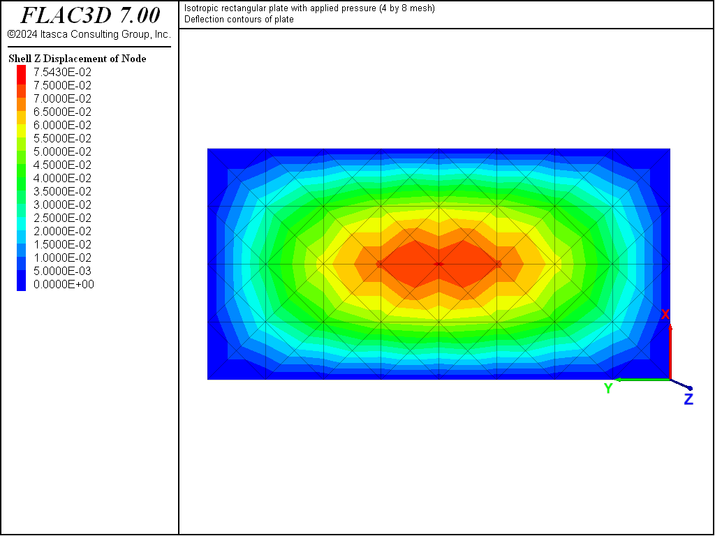
Figure 5: Deflection contours of isotropic plate.

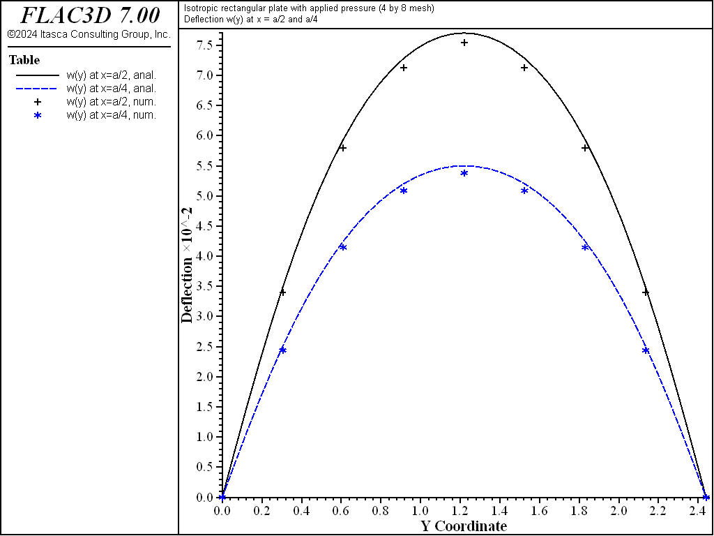
Figure 6: Deflection of isotropic plate along the lines \(x = a/2\) and \(x = a/4\).

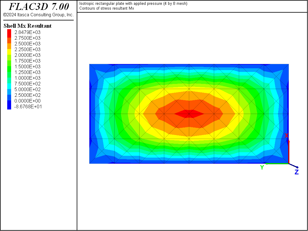
Figure 7: Stress resultant \(M_x\) contours of isotropic plate.

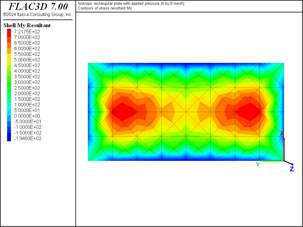
Figure 8: Stress resultant \(M_y\) contours of isotropic plate.

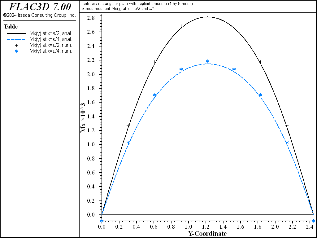
Figure 9: Stress resultant \(M_x\) of isotropic plate along the lines \(x = a/2\) and \(x = a/4\).

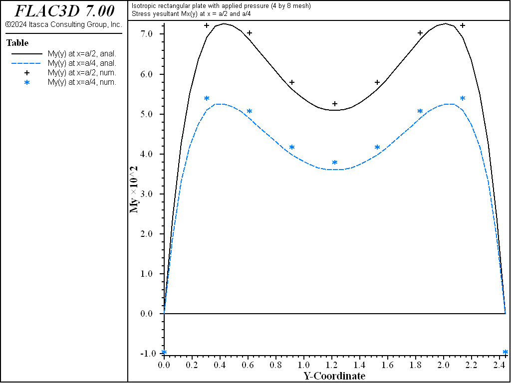
Figure 10: Stress resultant \(M_y\) of isotropic plate along the lines \(x = a/2\) and \(x = a/4\).

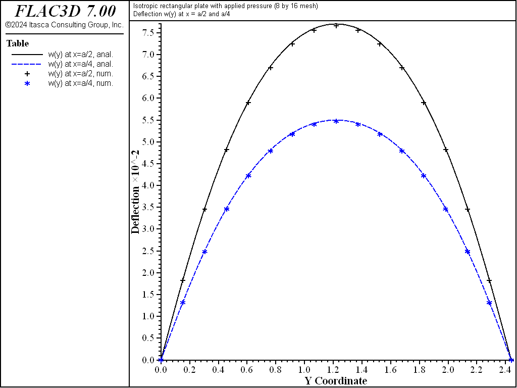
Figure 11: Deflection of isotropic plate along the lines \(x = a/2\) and \(x = a/4\) (8 by 16 mesh).

Orthotropic Case

The displacement field is shown in Figure 12 and Figure 13. The maximum deflection occurs at the plate center and equals 47.31 mm, which is within 5.1% of the theoretical value of 49.868 mm. A more refined 8 by 16 mesh gives a value of 49.50 mm, which is within 0.7% of the theoretical value. The deflection is compared with the theoretical solution along the lines \(x = a/2\) and \(x = a/4\) Figure 14. The bending stress resultant \(M_x\) and \(M_y\) fields are shown in Figure 15 and Figure 16, and compared with the theoretical solutions along the lines \(x = a/2\) and \(x = a/4\) in Figure 17 and Figure 18. The results are improved for a finer mesh (compare Figure 14 and Figure 19).

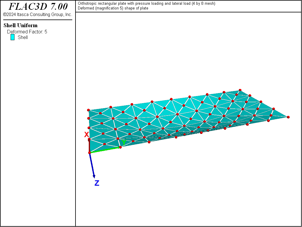
Figure 12: Deformed (magnification of 5) shape of orthotropic plate.

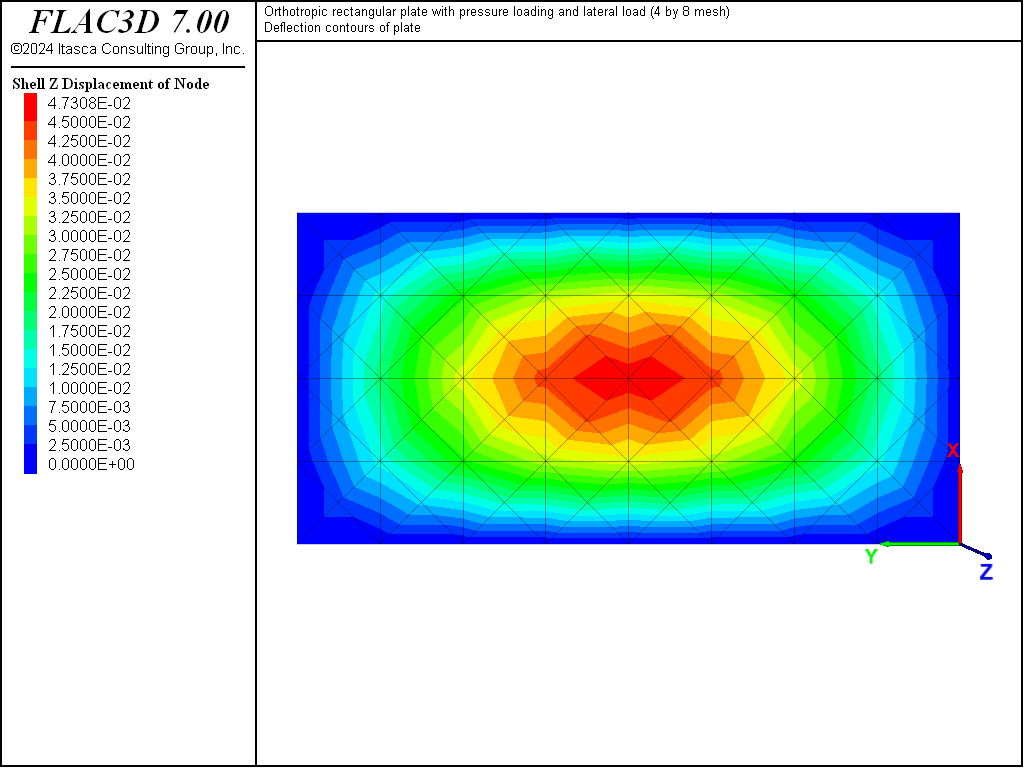
Figure 13: Deflection contours of orthotropic plate.

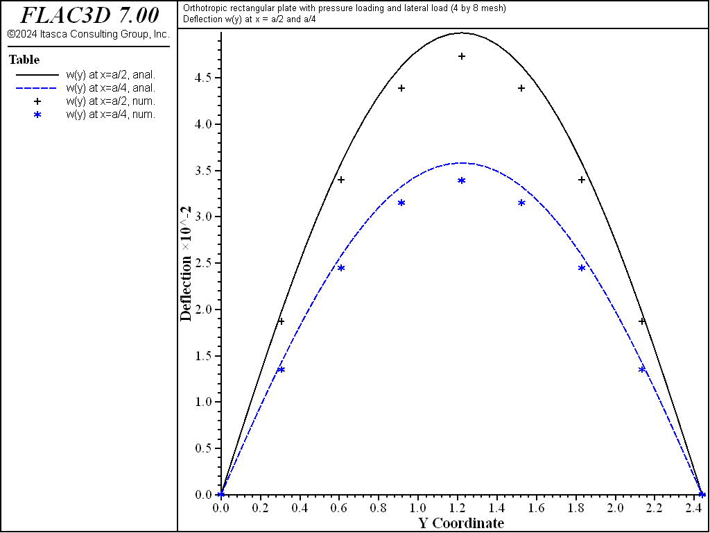
Figure 14: Deflection of orthotropic plate along the lines \(x = a/2\) and \(x = a/4\).

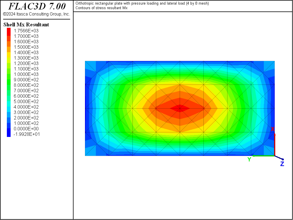
Figure 15: Stress resultant \(M_x\) contours of orthotropic plate.

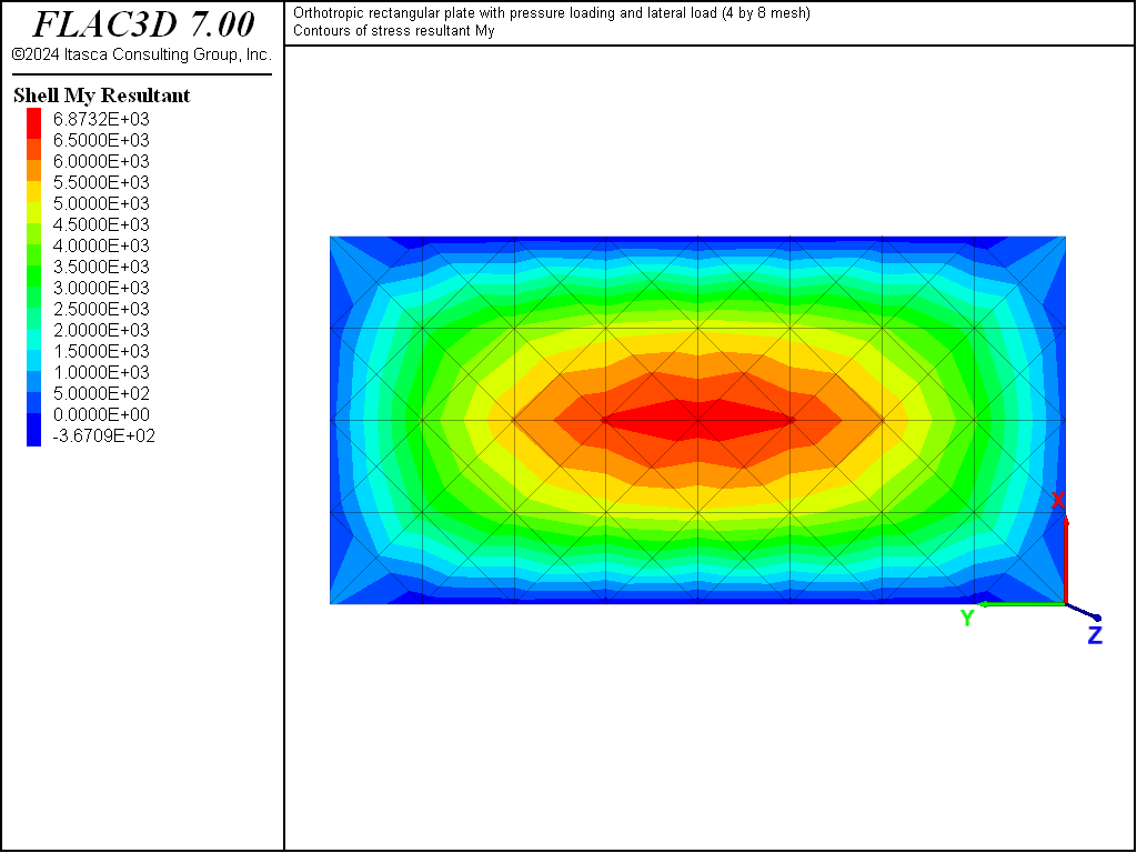
Figure 16: Stress resultant \(M_y\) contours of orthotropic plate.

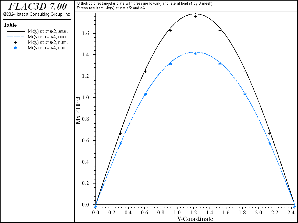
Figure 17: Stress resultant \(M_x\) of orthotropic plate along the lines \(x = a/2\) and \(x = a/4\).

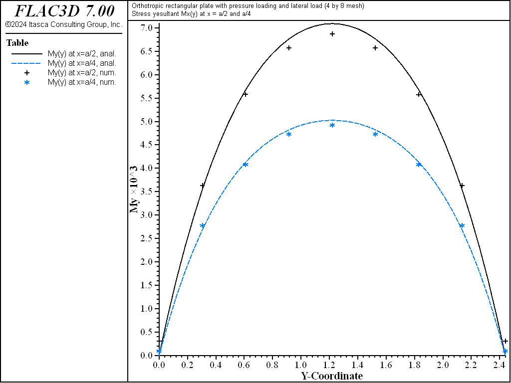
Figure 18: Stress resultant \(M_y\) of orthotropic plate along the lines \(x = a/2\) and \(x = a/4\).

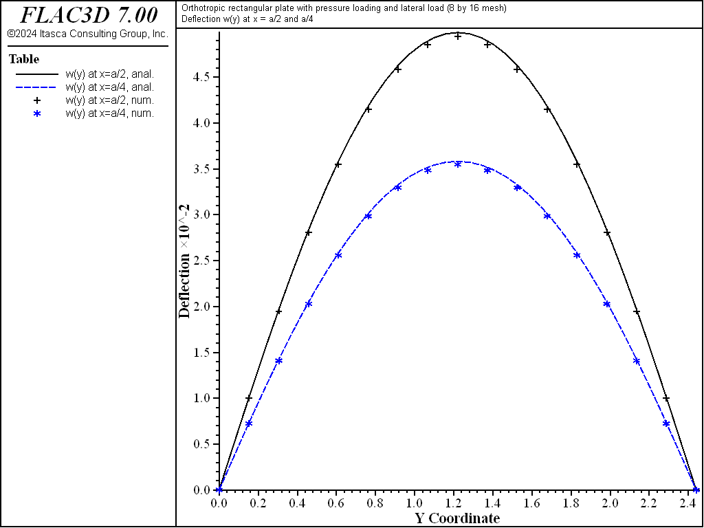
Figure 19: Deflection of orthotropic plate along the lines \(x = a/2\) and \(x = a/4\) (8 by 16 mesh).

Extending the System to Include Membrane Effects

The system described above only experiences bending loading. The orthotropic system was also subjected to a membrane loading by applying traction along the sheet boundary. Either the DKT-CST or the DKT-CST Hybrid element could be used, but in this case, the default DKT-CST element was used. In addition to the bending material stiffnesses (given in the equation above), we must also specify the membrane material stiffnesses, which can be approximated as follows.

The membrane material stiffnesses is chosen so that the membrane stiffness in both the \(x\)- and \(y\)-directions of a representative portion of the real sheet (shown in Figure 2) is the same as that of the orthotropic shell. The representative portion is a square with side length \(s\) in both the \(x\)- and \(y\)-directions (see Figure 20).

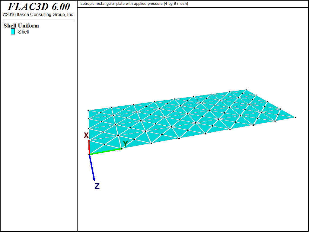
Figure 20: Representative portions of the sheet.

The membrane stiffnesses (\(AE/L\)) in the \(x\)- and \(y\)-directions for the real sheet and the orthotropic shell are

\[k_x = {{(st) E} \over s}, \ k_y = {{(st) E + (2wh)E^{\prime}} \over s} \ \ ({\rm real \ sheet})\]

\[k_x = {{(st) E_x} \over s} = tE_x, \ k_y = {{(st) E_y} \over s} = tE_y \ \ ({\rm orthotropic \ shell})\]

where \(s\), \(t\), \(E\), and \(E^{\prime}\) are defined in the equation above, and \(E_x\) and \(E_y\) are the effective moduli (Ugural 1981, p.141). The effective moduli are found by equating the corresponding stiffnesses:

\[E_x = E, \ E_y = E + \biggl({2wh \over st}\biggr)E^{\prime}\]

The orthotropic membrane stiffnesses required for input to FLAC3D are

\[{c^m_{11}}^{\prime} = {E_x \over {1 - \nu_x \nu_y}}\]

\[{c^m_{22}}^{\prime} = {E_y \over {1 - \nu_x \nu_y}}\]

\[{c^m_{33}}^{\prime} = G\]

\[{c^m_{12}}^{\prime} = {{E_x \nu_y} \over {1 - \nu_x \nu_y}} = {{E_y \nu_x} \over {1 - \nu_x \nu_y}}\]

where \(\nu_x\) and \(\nu_y\) are effective Poisson’s ratios, and \(G\) is shear modulus. This expression makes use of this equation from discussion of shell-element properties in the Structural Elements section. If we assume that \(\nu_x = \nu_y\) = 0 and \(G = E/2\), then:

\[{c^m_{11}}^{\prime} = 10 {\rm \ GPa}\]

\[{c^m_{22}}^{\prime} = 13.2 {\rm \ GPa}\]

\[{c^m_{33}}^{\prime} = 5 {\rm \ GPa}\]

\[{c^m_{12}}^{\prime} = 0\]

The system described above has a uniform membrane stress of 30 MPa that acts around the entire plate boundary. The edges at \(x\) = 0 and \(y\) = 0 are given roller boundary conditions, and the edges at \(x = a\) and \(y = b\) are loaded by using the structure node apply force-edge command with a value that takes into account the shell thickness. Each node receives the total force acting along its tributary area.[2] For these conditions, the stresses will be uniform throughout the plate and equal to

\[\sigma_{xx} = \sigma_{yy} = 30 \ {\rm MPa,} \ \ \tau_{xy} = 0\]

The displacements along the edges at \(x = a\) and \(y = b\) will be uniform and equal to

\[\Delta_x = \biggl({\sigma_m \over {c^m_{11}}^{\prime}}\biggr) a = 3.66 \ {\rm mm,} \ \ \Delta_y = \biggl({\sigma_m \over {c^m_{22}}^{\prime}}\biggr) b = 5.55 \ {\rm mm}\]

The results for a 4 by 8 mesh are as follows.

\[\sigma_{xx} = \sigma_{yy} = 30 \ {\rm MPa,} \ \ \tau_{xy} \approx 0\]

\[\Delta_x = 3.660 \ {\rm mm,} \ \ \Delta_y = 5.542 \ {\rm mm}\]

break

References

Cook, R. D., D. S. Malkus and M. E. Plesha. Concepts and Applications of Finite Element Analysis, Third Edition. New York: John Wiley & Sons Inc. (1989).

Ugural, A. C. Stresses in Plates and Shells. New York: McGraw-Hill Publishing Company Inc. (1981).

Data Files

isotropic4x8.dat

; FLAC3D isotropic plate with combined lateral & direct loads
; verification problem
model new
model large-strain off
model title "Isotropic rectangular plate with applied pressure (4 by 8 mesh)"
; Create the elements, and assign properties
struct shell create by-quadrilateral (0,0,0) (1.22,0,0) ...
                                     (1.22,2.44,0) (0,2.44,0) ...
                                     size (4,8) ...
                                     element-type=dkt cross-diagonal
struct shell property isotropic (10e9,0.0) thickness 19e-3
; simply supported condition - fix z velocity on all boundaries
struct node fix velocity-z range union position-x 0.0 position-x 1.22 ... 
                                       position-y 0.0 position-y 2.44
; Apply pressure loading
struct shell apply 19620
; Solve
model solve ratio-local=1e-5
; Save the result
model save 'isotropic4x8'

break

orthotropic4x8.dat

; FLAC3D orthotropic plate (bending) verification problem
model new
model large-strain off
[t =  'Orthotropic rectangular plate with pressure loading ']
[t += 'and lateral load (4 by 8 mesh)']
model title [t]
; ------------------------------------------------------------------------
struct shell create by-quadrilateral (0,0,0) (1.22,0,0) ...
                                     (1.22,2.44,0) (0,2.44,0) ...
                                     size (4,8) cross-diagonal
; Function to calculate orthotropic properties 
; given shell and stiffener properties
program call 'ortho_prop'
[ortho_prop(10e9,19e-3,0.0,25e-3,50e-3,10e9,0.41)]
struct shell property orthotropic-bending [bend_stiff] ...
                      orthotropic-membrane [memb_stiff] ...
                      material-x (1,0,0) thickness 19e-3
; simply supported condition
struct node fix velocity-z range union position-x 0 position-x 1.22 ...
                                       position-y 0 position-y 2.44
; Apply membrane loading - edge loading
struct node apply force-edge (5.7e5,0,0) range position-x 1.22
struct node apply force-edge (0,5.7e5,0) add range position-y 2.44
; Apply rollers to the other edges
struct node fix velocity-x range position-x 0 
struct node fix velocity-y range position-y 0 
; Apply pressure loading
struct shell apply 19620
; Solve
model solve ratio-local=1e-5
; Save
model save 'orthotropic4x8'

ortho_prop.dat

; Calculate orthotropic shell properties given 
;    e = shell young's modulus,
;    t = shell thickness, 
;    nu = shell Poisson's ratio, 
;    swidth = stiffener width,
;    sheight = stiffener height, 
;    se = stiffener stiffness, and 
;    sspace = stiffener spacing
; Returns 4x1 arrays with membrane and bending stiffness 
; in globals memb_stiff and bend_stiff.
; Also flexural rigidities in global map rigidity
fish automatic-create off
fish define ortho_prop(e,t,nu,swidth,sheight,se,sspace)
    global rigidity = map
    rigidity('Dxy') = 0.0
    rigidity('Dx')  = e * t^3 / (12.0*(1.0 - nu^2))
    rigidity('H')   = rigidity('Dx')
    rigidity('Gxy') = (rigidity('H') - rigidity('Dxy')) / 2.0
    local Iv = swidth*sheight*sheight*sheight / 12.0
          Iv = Iv + (swidth*sheight*(t + sheight)^2) / 4.0
          Iv = 2.0 * Iv
    rigidity('Dy') = rigidity('Dx') + (se * Iv) / sspace
    
    global bend_stiff = matrix(4,1)
    bend_stiff(1,1) = (12.0 / t^3) * rigidity('Dx')
    bend_stiff(2,1) = (12.0 / t^3) * rigidity('Dxy')
    bend_stiff(3,1) = (12.0 / t^3) * rigidity('Dy')
    bend_stiff(4,1) = (12.0 / t^3) * rigidity('Gxy')
    
    ; Membrane stiffness, only used for membrane.f3dat
    global memb_stiff = matrix(4,1)
    memb_stiff(1,1) = e
    memb_stiff(2,1) = 0.0
    memb_stiff(3,1) = e + (2.0 * swidth * sheight / (sspace * t)) * se
    memb_stiff(4,1) = e / 2.0
end

Endnotes

[1]	To view this project in FLAC3D, use the program menu. Help ▼ Examples…   ⮡   FLAC     ⮡   VerificationProblems       ⮡   SimplySupportedOrthotropicPlate         ⮡   SimplySupportedOrthotropicPlate.prj

[2]	For a system experiencing combined membrane and bending loads, a shell element (such as the DKT-CST) must be used. In order to model the coupling whereby the presence of a tensile membrane force decreases the plate deflection, FLAC3D must be run in large-strain mode.