Formulation of a 3D Explicit Finite Volume Model
FLAC3D is an explicit finite volume program to study, numerically, the mechanical behavior of a continuous three-dimensional medium as it reaches equilibrium or steady plastic flow. The response observed derives from a particular mathematical model on one hand, and from a specific numerical implementation on the other. These two topics are addressed below.
Mathematical Model Description
The mechanics of the medium are derived from general principles (definition of strain, laws of motion), and the use of constitutive equations defining the idealized material. The resulting mathematical expression is a set of partial differential equations, relating mechanical (stress) and kinematic (strain rate, velocity) variables, which are to be solved for particular geometries and properties, given specific boundary and initial conditions.
An important aspect of the model is the inclusion of the equations of motion, although FLAC3D is primarily concerned with the state of stress and deformation of the medium near the state of equilibrium. The numerical implementation section shows that the inertial terms are used as a means by which to reach the equilibrium state in a numerically stable manner.
Conventions
In the Lagrangian formulation adopted in FLAC3D, a point in the medium is characterized by the vector components \(x_i\), \(u_i\), and \(dv_i\) \(/\ dt\), \(i\) = 1,3 of position, displacement, velocity and acceleration, respectively.
As a notation convention, a bold letter designates a vector or tensor, depending on the context. The symbol \(a_i\) denotes component \(i\) of the vector [\(a\)] in a Cartesian system of reference axes; \(A_{ij}\) is component (\(i,j\) ) of tensor [\(A\)]. Also, \(α_i\) is the partial derivative of \(α\) with respect to \(x_i\). (\(α\) can be a scalar variable, a vector or tensor component.)
By definition, tension and extension are positive.
The Einstein summation convention applies, but only on indices \(i\), \(j\) and \(k\), which take the values 1, 2, 3.
Stress
The state of stress at a given point of the medium is characterized by the symmetric stress tensor \(σ_{ij}\). The traction vector [\(t\)] on a face with unit normal [\(n\)] is given by Cauchy’s formulae (tension positive):
Rate of Strain and Rate of Rotation
Let the particles of the medium move with velocity [\(v\)]. In an infinitesimal time, \(dt\), the medium experiences an infinitesimal strain determined by the translations \(v_i\)\(dt\), and the corresponding components of the strain-rate tensor may be written as
where partial derivatives are taken with respect to components of the current position vector [\(x\)].
For later reference, the first invariant of the strain-rate tensor gives a measure of the rate of dilation of an elementary volume. Aside from the rate of deformation characterized by the tensor \(ξ\)\(ij\), a volume element experiences an instantaneous rigid-body displacement, determined by the translation velocity [\(v\)], and a rotation with angular velocity.
where \(e_{ijk}\) is the permutation symbol, and [\(ω\)] is the rate of rotation tensor whose components are defined as
Equations of Motion and Equilibrium
Application of the continuum form of the momentum principle yields Cauchy’s equations of motion:
where \(ρ\) is the mass-per-unit volume of the medium, [\(b\)] is the body force per unit mass, and \(d\)[\(v\)]/\(dt\) is the material derivative of the velocity. These laws govern, in the mathematical model, the motion of an elementary volume of the medium from the forces applied to it. Note that, in the case of static equilibrium of the medium, the acceleration \(d\)[\(v\)]/\(dt\) is zero, and Equation (5) reduces to the partial differential equations of equilibrium:
Boundary and Initial Conditions
The boundary conditions consist of imposed boundary tractions (see Equation (1)) and/or velocities (to induce given displacements). In addition, body forces may be present. Also, the initial stress state of the body needs to be specified.
Constitutive Equations
The equations of motion Equation (5), together with the definitions (Equation (2)) of the rates of strain, constitute nine equations for fifteen unknowns (the 6 + 6 components of the stress- and strain-rate tensors and the three components of the velocity vector). Six additional relations are provided by the constitutive equations that define the nature of the particular material under consideration. They are usually given in the form
in which \([\check \sigma]\) is the corotational stress-rate tensor, [\(H\)] is a given function, and \(κ\) is a parameter that takes into account the history of loading. The corotational stress rate \([\check \sigma]\) is equal to the material derivative of the stress as it would appear to an observer in a frame of reference attached to the material point and rotating with it at an angular velocity equal to the instantaneous value of the angular velocity [\(Ω\)] of the material. Its components are defined as
in which \(dσ_{ij}\)/\(dt\) is the material time derivative of [\(σ\)], and [\(ω\)] is the rate of rotation tensor.
Numerical Formulation
The method of solution in FLAC3D is characterized by the following three approaches:
- finite volume approach (First-order space and time derivatives of a variable are approximated by finite volumes assuming linear variations of the variable over finite space and time intervals, respectively.);
- discrete-model approach (The continuous medium is replaced by a discrete equivalent — one in which all forces involved (applied and interactive) are concentrated at the nodes of a three-dimensional mesh used in the medium representation.); and
- dynamic-solution approach (The inertial terms in the equations of motion are used as numerical means to reach the equilibrium state of the system under consideration.)
The laws of motion for the continuum are, by means of these approaches, transformed into discrete forms of Newton’s law at the nodes. The resulting system of ordinary differential equations is then solved numerically using an explicit finite difference approach in time.
The spatial derivatives involved in the derivation of the equivalent medium are those appearing in the definition of strain rates in term of velocities. For the purpose of defining velocity variations and corresponding space intervals, the medium is discretized into constant strain-rate elements of tetrahedral shape whose vertices are the nodes of the mesh mentioned above. A tetrahedron is represented in Figure 1, as an illustration:

Figure 1: Tetrahedron
Finite Volume Approximation to Space Derivatives
The finite volume formulation of the strain-rate tensor components for the tetrahedron are derived below as a preliminary to the nodal formulation of the equations of motion. The tetrahedron nodes are referred to locally by a number from 1 to 4 and, by convention, face \(n\) is opposite node \(n\). (See Figure 1.)
By application of the Gauss divergence theorem to the tetrahedron, we can write
where the integrals are taken over the volume and the surface of the tetrahedron, respectively, and [\(n\)] is the exterior unit vector normal to the surface.
For a constant strain-rate tetrahedron, the velocity field is linear, and [\(n\)] is constant over the surface of each face. Hence, after integration, Equation (9) yields
where the superscript ( \(f\) ) relates to the value of the associated variable on face \(f\), and \({\overline{v_i}}\) is the average value of velocity component \(i\). For a linear velocity variation, we have
where the superscript \(l\) relates to the value at node \(l\).
Substitution of Equation (11) in (10) yields, reorganizing terms by node contribution,
If we replace \(v_i\) with 1 in Equation (9) we obtain, by application of the divergence theorem,
Using this last relation, and dividing Equation (12) by \(V\), we get
and the components of the strain-rate tensor may be expressed as
Nodal Formulation of the Equations of Motion
The nodal formulation of the equations of motion will be derived below by application of the theorem of virtual work, at any instant in time, to an equivalent static problem. Approximations on the form of the nodal inertial terms will be made by using those terms as means to reach the solution corresponding to the equilibrium equations, Equation (6).
Fixing time, \(t\), we consider an equivalent static problem governed at any instant in time by the equilibrium equations
with body forces defined as (Equation (5))
In the framework of the finite volume approximation adopted here, the medium is represented by a continuous assembly of constant-strain tetrahedra subjected to body forces \([B]\). The nodal forces \([f]^n\), with \(n\) = (1,4), acting on a single tetrahedron in “static” equilibrium with the tetrahedron stresses and equivalent body forces, are derived by application of the theorem of virtual work. After application of a virtual nodal velocity \(δ[v]^n\) (it will generate a linear velocity field \(δ[v]\) and a constant strain-rate \(δ[ξ]\) inside the tetrahedron), we equate the external rate of work done by the nodal forces \([f]^n\) and body forces \([B]\) with the internal work rate done by the stresses \(σ_{ij}\) under that velocity.
Following the notation conventions (a superscript refers to the nodal value of a variable) and Einstein summation convention on indices \(i\) and \(j\), the external work rate may be expressed as
while the internal work rate is given by
Using Equation (15), we can write, for a constant strain-rate tetrahedron,
The stress tensor is symmetric and, defining a vector \(T^l\) with components
we obtain
After substitution of Equation (17) in (18), the external work rate may be expressed as
where \(E^b\) and \(E^I\) are the external work-rate contributions of the body forces \(ρb_i\) and inertial forces, respectively. For a constant-body force \(ρb_i\) inside the tetrahedron, we can write
while \(E^I\) may be expressed as
According to the finite volume approximation done earlier, the velocity field varies linearly inside the tetrahedron. To describe it, we adopt a local system of reference axes \(xʹ\)1, \(xʹ\)2, \(xʹ\)3, with origin at the tetrahedron centroid, and write
where \(N^n\) (with \(n\) = 1,4) are linear functions of the form
and \(c^n_0\), \(c^n_1\), \(c^n_2\), \(c^n_3\) (with \(n\) = 1,4) are constants determined by solving the systems of equations
where \(δ_{nj}\) is the Kronecker delta. By definition of the centroid, all integrals of the form \(\int_V {x'}_j dV\) vanish, and substitution of Equation (26) for \(δv_i\) in Equation (24) yields, using Equation (27),
Using Cramer’s rule to solve Equation (28) for \(c^n_0\), we obtain, taking advantage of the properties of the centroid,
From Equation (29) and (30), we may write
Also, substitution of Equation (26) for \(δv_i\) in Equation (25) gives
Finally, with expressions Equation (31) for \(E^b\) and Equation (32) for \(E^I\), Equation (23) becomes
For static equilibrium of the tetrahedron in the framework of the equivalent problem, the internal work rate (see Equation (22)) equals the external work rate expressed by Equation (33) for any virtual velocity. Hence, we must have, regrouping terms,
For small spatial variations of the acceleration field around an average value inside the tetrahedron, the last term in Equation (34) may be expressed as
Also, for constant values of \(ρ\) inside the tetrahedron, and using the properties of the centroid mentioned above (see Equation (27) and (30)) we may write
In the context of this analysis, the mass \(ρV\)/4 involved in the inertial term above is replaced by a fictitious nodal mass \(m^n\), whose value will be determined below, in order to ensure numerical stability of the system on its route to equilibrium. Accordingly, Equation (36) becomes
and Equation (34) may be written as
The equilibrium conditions for the equivalent system may now be established by requiring that, at each node, the sum of the statically equivalent forces, -[\(f\)], of all contributing tetrahedra and nodal contributions [\(P\)] of applied loads and concentrated forces be zero. To express those conditions, we adopt a notation where a variable with superscript <\(l\)> refers to the value of the variable at a node with label \(l\) in the global node numbering. The symbol [[.]]\(^{<l>}\) is used to represent the sum of the contributions at global node \(l\) of all tetrahedra meeting at that node. With those conventions, we may write the following expressions of Newton’s law at the nodes:
where \(n_n\) is the total number of nodes involved in the medium representation, the nodal mass \(M^{<l>}\) is defined as
and the out-of-balance force \([F]^{<l>}\) is given by
This force is equal to zero when the medium has reached equilibrium.
Explicit Finite Difference Approximation to Time Derivatives
Taking into consideration the constitutive equations, Equation (7), and the relation Equation (15) between deformation rate and nodal velocities, Equation (39) may be expressed formally as a system of ordinary differential equations of the form
where the notation {}\(^{<l>}\) refers to the subset of nodal velocity values involved in the calculation at global node \(l\) (see Equation (39)) In FLAC3D, this system is solved numerically using an explicit finite difference formulation in time. In this approach, the velocity of a material node is assumed to vary linearly over a time interval \(Δt\), and the derivative on the left-hand side of Equation (42) is evaluated using central finite differences, whereby velocities are stored for times that are displaced by half-timesteps with respect to displacements and forces. Nodal velocities are computed using the recurrence relation
In turn, the node location is similarly updated using the central finite difference approximation,
First-order error terms vanish when the finite difference scheme embodied in Equation (43) and (44) is used (i.e., the scheme is second-order accurate).
Nodal displacements are calculated in the code from the relation
with \(u_i^{<l>}(0) =0\).
Constitutive Equations in Incremental Form
In FLAC3D, it is assumed that velocities remain constant in the time interval, \(Δt\). An incremental expression of the constitutive Equation (7) with the following form is used:
where \(\Delta \check\sigma_{ij}\) is the corotational stress increment, and \(H^*_{ij}\) is a given function.
For small displacements and displacement gradients during \(Δt\), we may write
where \(Δ_{ij}\) is the change of strain related to the configuration at time \(t\).
The stress increment \(Δσ_{ij}\) is computed from \(\Delta{\check{\sigma}}_{ij}\), using
where \(Δσ^C_{ij}\) is a stress correction defined as (see Equation (8))
The components of the rate-of-rotation tensor are calculated using Equation (4) and the finite difference formulation Equation (14):
Specific forms of the constitutive function \(H^*\) are described in Constitutive Models, where the subject of their numerical implementation in FLAC3D is also discussed.
Large- and Small-Strain Modes
The numerical formulation described above provides a description of large-strain deformation, involving large displacements, displacement gradients and rotations. This is termed the large-strain mode in FLAC3D.
In applications in which the rotations are sufficiently small that the components \(ω_{ij}\) - \(δ_{ij}\) are small compared to unity, [\(ω\)] may be replaced by [\(I\)], and the stress correction in Equation (48) may be omitted. Also, for small displacements and displacement gradients, the spatial derivatives involved in the definition Equation (2) of the strain-rate tensor may be evaluated with respect to the initial configuration, and the node coordinates need not be updated (see Equation (44)).
In FLAC3D, the small-strain mode assumes small displacements, displacement gradients and rotations. In that mode, node coordinates are not updated, and stress rotation corrections are not taken into consideration.
Mechanical Timestep Determination for Numerical Stability
The difference equations (Equation (43)) will not provide valid answers unless the numerical scheme is stable. Some physical insight on this topic may be gained by viewing the idealized medium as an assembly of point masses (located at the nodes) connected by linear springs, a conceptualization which may be made on the following grounds. The equations of motion for a mass-spring system may be expressed, in matrix notation, as
where the braces denote vectors of nodal values, {\(P*\)} are exterior forces, [\(K\)] is the matrix of rigidity of the springs, and [\(M\) ] is a diagonal nodal mass matrix. The analogy with the idealized medium is immediate if we interpret the out-of-balance forces in Equation (39) as the applied and spring reaction forces in Equation (51).
In studying the oscillating mass-spring system with a finite difference scheme, a timestep that does not exceed a critical timestep related to the minimum eigenperiod of the total system must be used. Hence, the stability criterion for the numerical scheme must provide an upper bound for the values of the timesteps used in the finite difference scheme.
Derivation of a relation providing a measure of critical timesteps for the system requires knowledge of the eigenperiods of the system. However, in practice, global eigenvalue analyses are impractical and not commonly used for this purpose (see Press et al. 1986). In FLAC3D, as will be shown below, a local variation of this stability analysis is performed. An important aspect of the numerical method is that a uniform unit timestep \(Δt\) is adopted for the whole system:
And the nodal masses on the right-hand side of Equation (39) are taken as variables, and adjusted to fulfill the local stability conditions.
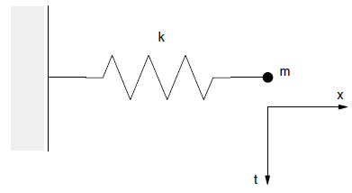
Figure 2: Mass-spring system 1.
First, consider the one-dimensional mass-spring system represented in Figure 2. The motion of the point mass, with a given initial displacement, is governed by the differential equation
where \(k\) is the stiffness of the spring, and \(m\) is the point mass. The critical timestep corresponding to a second-order finite difference scheme for this equation is given by (Bathe and Wilson 1976):
where \(T\) is the period of the system — i.e.,
[CS: found this snippet here, and don’t know why. Leaving it (hidden) in place until mystery resolved:: Stubby stub. Section 1.2 (+ subsections) from theory here.]
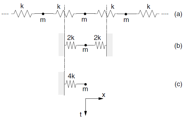
Figure 3: Mass-spring system 2.
Now consider the infinite series of masses and springs in Figure 3-a. By symmetry, the behavior of this assembly may be analyzed by studying the system sketched in Figure 3-b which, in turn, is equivalent to a single mass-spring system with stiffness 4\(k\) (Figure 3-c) The limit-stability criterion, derived from Equation (54) and (55), has the form
By selecting \(Δt\) = 1, the system will be stable if the magnitude of the point mass is greater than or equal to the spring stiffness. In the local analysis, the validity of (56) is extended to one tetrahedron by interpreting \(m\) as the nodal mass contribution, \(m^l\), at local node, \(l\), and \(k\) as the corresponding nodal stiffness contribution, \(k^l\). The nodal mass contribution as derived from the infinite series criterion provides an upper-bound value for the system under consideration. The nodal stiffness contribution is derived from a simple diagonalization technique of the local stiffness matrix, as follows.
The tetrahedron internal-force contribution at local node \(l\) is equal to \(T^l_{i}\)/3 (see Equation (41)) This force is interpreted as a spring reaction force of the form \(-k^l_{ij}\)\(u^l_{j}\) (see Equation (51)) Taking variations over a time interval, \(dt\), we write
Using (21), this relation becomes
With a unit-velocity component in direction \(q\) at node \(l\), and all other nodal velocity components set to zero, we obtain from Equation (58) the diagonal terms of the local stiffness matrix
where, by convention, no summation is implied on repeated index \(q\), which runs from 1 to 3.
Adopting the small-strain incremental form of Hooke’s law to describe the stress-strain constitutive relation in the small time interval, we write
in which \(α\)1 = \(K\) + 4/3\(G\), \(K\) is the bulk modulus and \(G\) is the shear modulus.
Using the selected nodal-velocity values in the finite difference formulation Equation (15) for \(ξ\), we have
Substitution of this expression in Equation (60) gives
We now define an upper-bound value for the nodal stiffness contribution as
which yields, from Equation (56) with Equation (52), the expression for the tetrahedron mass contribution at node \(l\):
to provide a numerically stable solution.
Mechanical Damping
The equations of motion must be damped to provide static or quasi-static (non-inertial) solutions.
Local nonviscous damping is the default damping algorithm for static analysis in FLAC3D,
and is described in this section.
Local damping can be controlled with the zone mechanical damping local <f> command,
where f is the local damping (default is 0.8).
Local damping can also be implemented in a dynamic analysis
(see the section Dynamic Analysis).
An alternative damping algorithm is provided in FLAC3D for situations
in which the steady-state solution includes a significant uniform motion.
This can occur, for example, in a creep simulation, or in the calculation of the ultimate capacity of an axially loaded pile.
This damping is called combined damping, and is also described in this section.
Combined damping is more efficient than local damping at removing kinetic energy for this special case.
Combined damping is invoked with the zone mechanical damping combined <f> command.
For dynamic analyses, Rayleigh damping and artificial viscosity damping are also available to control damping. These algorithms are described in the section on Mechanical Damping in the Theory and Background section.
Local Nonviscous Damping
The local nonviscous damping used in FLAC3D is similar to that described in Cundall (1987). A damping-force term is added to the equations of motion, given by Equation (39), such that the damped equations of motion can be written as
\(\mathcal{F}_{(i)}^{<l>}\) is the damping force and is given by
expressed in terms of the generalized out-of-balance force, \(F^{<l>}_i\), and the generalized velocity, \(v^{<l>}_{(i)}\). The damping force is controlled by the damping constant, \(α\), whose default value is 0.8.
This form of damping has three advantages:
- Only accelerating motion is damped; therefore, no erroneous damping forces arise from steady-state motion.
- The damping constant, \(α\), is nondimensional.
- Since damping is frequency-independent, regions of the assembly with different natural periods are damped equally, using the same damping constant.
The local nonviscous damping formulation in FLAC3D is similar to hysteretic damping, in which the energy loss per cycle is independent of the rate at which the cycle is executed. This similarity is demonstrated in the following analysis.
Upon examination of Equation (66), it is evident that the damping force always opposes motion, but it is scaled to the resultant generalized force, unlike viscous damping, which is scaled to the magnitude of velocity. Two forms of Equation (66) may be written, depending on the relative signs of \(F_i^{<l>}\) and \(v_{(i)}^{<l>}\). When they are of the same sign, the equation of motion is
and when they are of opposite signs, the equation of motion is
These equations may be written in terms of apparent mass as
where \(\mathcal{M}^+ = {M^{<l>} / (1-\alpha)}\) and \(\mathcal{M}^- = {M^{<l>} / (1+\alpha)}\).
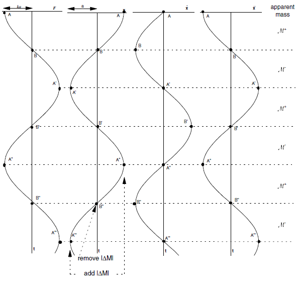
Figure 4: Motion of single mass-spring system.
The motion of the single degree-of-freedom mass-spring system from Figure 2, when given an initial displacement such that \(x = a\) at \(t\) = 0, is shown in Figure 4. For such motion, the apparent mass is increased at the two times in each cycle when the velocity is zero, and reduced at the two times when the velocity is maximum. The damping operates by removing kinetic energy twice per cycle: at the two points of peak velocity, part of the moving mass is removed and discarded. Note that there is no discontinuity in acceleration, since the acceleration is zero at the instant when mass is removed.
The amount of energy removed per cycle is given by twice the drop in kinetic energy at point \(B\), or
and the mean kinetic energy at the instant of removal is
where \(v_{(i)}^{<l>}\) is the generalized velocity given by Equation (66).
The ratio of energy lost per cycle to maximum energy stored is called the “specific loss” (Kolsky 1963). The specific loss can be written in terms of the damping constant in FLAC3D by noting that, for a single degree-of-freedom system, or for oscillation in a single mode, the peak kinetic energy is the same as the peak stored energy. Thus, the specific loss can be written as
The fraction of critical damping, \(D\), can be written in terms of the specific loss for small values of damping as
For the default value of \(α\) = 0.8, the approximate fraction of critical damping is therefore 0.25.
Equation (72) can be verified by loading one zone and a column of three zones, respectively, with a suddenly applied gravity load and allowing each system to oscillate to equilibrium. Both tests give approximately the same value for \(Δ W/W\), confirming that the damping is independent of frequency. However, for a system where multiple modes are active simultaneously, the response computed by FLAC3D may not show the same damping for each mode.
Combined Damping
The damping formulation described by Equation (66) is only activated when the velocity component changes sign. In situations where there is significant uniform motion (in comparison to the magnitude of oscillations that are to be damped), there may be no “zero crossings,” and hence no energy dissipation. An alternative (but less efficient) formulation is derived by noting that, for a single degree-of-freedom system executing harmonic motion, the derivative of the unbalanced force is proportional to minus the velocity. If
then
Hence \({d F \over dt}\) is proportional to \(v\). However, the mean value of \({d F \over dt}\) is zero even when the mean value of \(v\) is nonzero, for an oscillating system. An alternative form of damping called “combined damping,” is provided in FLAC3D. The scheme consists of a damping force composed of equal contributions from expressions based on velocity and \({d F \over dt}\):
This form of damping should be used if there is significant rigid-body motion of a system in addition to oscillatory motion to be dissipated. However, combined damping is found to dissipate energy at a slower rate than local damping based on velocity. Therefore, local damping is preferred in most cases.
The effect of rigid-body motion is demonstrated in ElasticBlock.dat, which models a block under gravity. The corresponding project file is “ElasticBlock.prj,” located in “datafiles\theory\elastic-block.” However, the lower boundary is constrained to move upwards at constant velocity, and all gridpoints are fixed in the horizontal direction. The final “equilibrium” state should be one in which gravity-induced stresses act in the body but, in addition, all gridpoints should move upwards at the same velocity. As seen from the velocity history of one top-surface gridpoint (shown in Figure 5), the body continues to oscillate indefinitely and does not reach the predicted steady state.
ElasticBlock.dat
model new
model large-strain off
fish automatic-create off
zone create brick size 5 5 5
zone cmodel elastic
zone property shear 1 bulk 2
zone initialize density 1
model gravity 0 0 -10
zone gridpoint fix velocity-x
zone gridpoint fix velocity-y
zone gridpoint fix velocity range position-z 0
zone gridpoint initialize velocity-z 1.0
history interval 10
zone history velocity-z position 3 3 5
model save 'ini'
;
model step 1000
model save 'undamped'
;
model restore 'ini'
zone mechanical damping combined
model step 1000
model save 'damped'
;
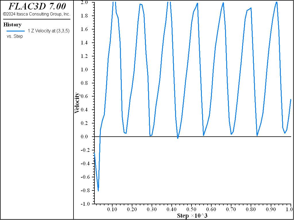
Figure 5: z-velocity history at top of block — local damping.
When the zone mechanical damping combined command is specified,
the system then converges to the steady state in which all velocities are equal to the imposed velocity
(see Figure 6),
and the internal stresses exhibit the same gravitational gradient as the static case.
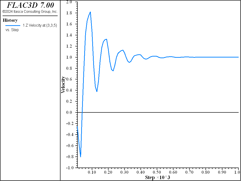
Figure 6: z-velocity history at top of block — combined damping.
| Was this helpful? ... | FLAC3D © 2019, Itasca | Updated: Feb 25, 2024 |