One-Dimensional Earthquake Excitation of a Uniform Layer
Note
To view this project in FLAC3D, use the menu command . Choose “Dynamic/EarthquakeExcitation” and select “EarthquakeExcitation.prj” to load. The main data files are shown at the end of this example. The remaining data files can be found in the project.
An example of a 20 m layer excited by a digitized earthquake is provided to show that plausible behavior occurs when using hysteretic damping for a case involving wave propagation, multiple and nested loops, and reasonably large cyclic strain.
The digitized earthquake record is imported from the file described as “gilroy1.acc”. The stress/strain loops for the bottom and middle of the layer are shown in Figure 1 and Figure 2, respectively, and the acceleration histories for three positions are shown in Figure 3 through Figure 5. The simulation is in one dimension, for excitation in the shear direction only. Note that for this example, the initial stresses are zero. If a nonzero initial vertical and horizontal stress state is specified, then the left and right boundaries should be attached to produce a one-dimensional simulation.
The hysteretic model seems to handle multiple nested loops in a reasonable manner. There is clearly more energy dissipation at the base of the model than at the middle. The maximum cyclic strain is about 0.1%. The magnitude of timestep is unaffected by the hysteretic damping.
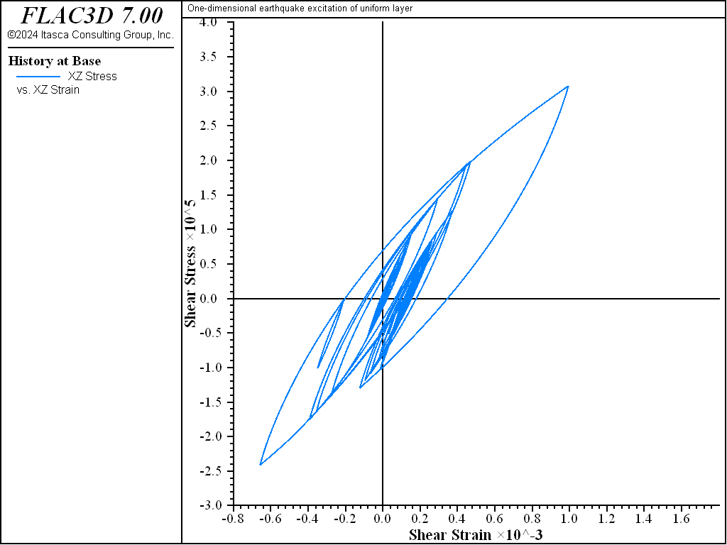
Figure 1: Shear stress vs shear strain for base of the layer; default FLAC3D hysteretic model.
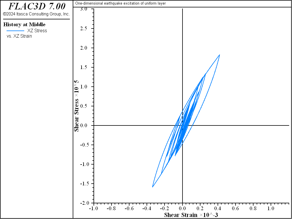
Figure 2: Shear stress vs shear strain for middle of the layer; default FLAC3D hysteretic model.
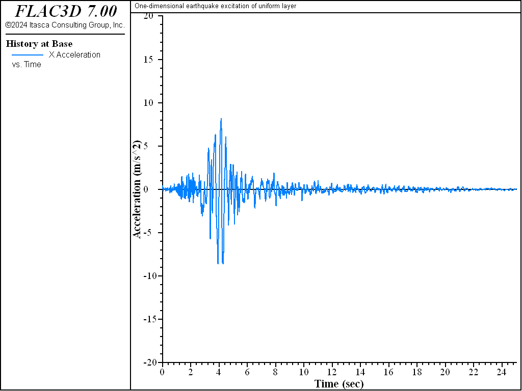
Figure 3: Acceleration history for base of layer vs time (sec).
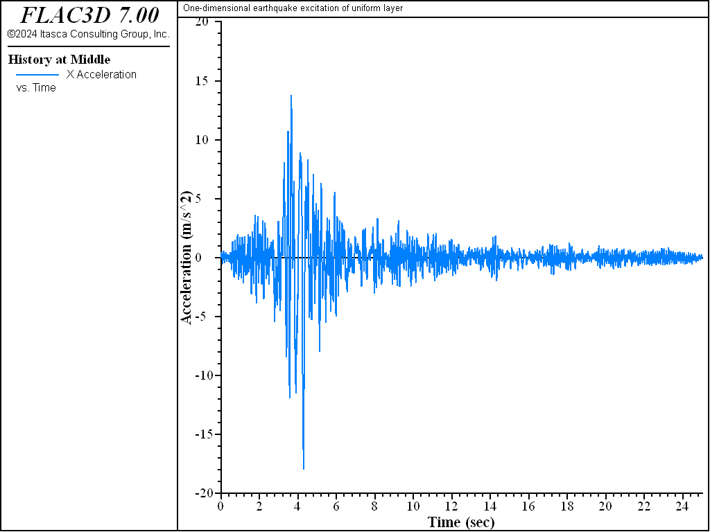
Figure 4: Acceleration history for middle of layer vs time (sec).
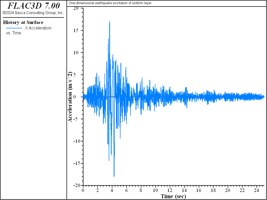
Figure 5: Acceleration history for surface of layer vs time (sec).
Check initial shear stress state — In laboratory tests, the initial shear stress is assumed to be zero, leading to hysteresis loops that are generally symmetrical. In practical applications, the initial shear stress is unlikely to be zero (for example, within soil elements near the surface of an embankment). The user of hysteretic damping must decide on the best estimate of the initial state of the material, because the hysteretic formulation in FLAC3D depends on the past history of shear strain. Two cases can be identified:
- If hysteretic damping is activated after a set of equilibrium stresses has been installed, then the initial shear strain will be zero, and cyclic excursions of shear stress will tend to be symmetrical about the starting point.
- If the initial stresses are built up by straining the model while hysteretic damping is active, then subsequent cyclic excursions of shear stress will tend to be asymmetrical because the initial bias in strain causes the slope of the stress/strain curve to be flatter on the side with higher stress.
These cases are illustrated by modifying this simple application. With no initial shear stress, the cyclic response of the model is nearly symmetrical, as shown in Figures 1 and 2.
The simulation is repeated with uniform shear stresses of 0.1 MPa initialized in the 20 m layer, and with an equal static shear stress applied at the boundary to maintain initial equilibrium. The following commands are added to the data file.
; Initial conditions
zone initialize stress-xz 1e5
and, in the boundary condition section:
zone face apply stress-xz 1e5 range union position-z=0 position-z=20
The resulting dynamic response is identical to that of the original simulation, but the set of loops is shifted upward by 0.1 MPa. Figure 6 shows the result at the base of the model; compare to Figure 1. This corresponds to Case 1 above.
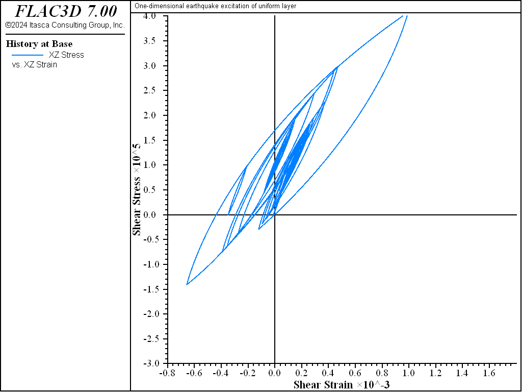
Figure 6: Shear stress vs shear strain for base of the layer; with shear stress simply initialized to 0.1 MPa.
In order to make the initial strains compatible with the initial stresses, hysteretic damping is arranged to be active during the establishment of the initial stress state. For this case, the following commands are added to the data file, in the section where boundary conditions are being applied.
zone face apply stress-xz 1e5 range union position-z=0 position-z 20
; Solve to equilibrium with hysteretic damping active
zone dynamic damping hysteretic default -3.325 0.823
zone dynamic damping local 0.7
model solve
; Reset model
zone gridpoint initialize velocity (0,0,0)
zone dynamic time-total 0
zone dynamic damping local 0.0
Shear stresses are applied to the boundaries of the grid, but not initialized within the grid. Thus, a static solution (using additional local damping with the hysteretic damping to speed convergence) is used to build up internal stresses. Because hysteretic damping is active during the static solution, strains will be compatible with stresses at the start of the dynamic simulation. The dynamic response of the system is indicated by the stress/strain loops plotted in Figure 7. In this case there is a marked asymmetry. The soil is already partially yielded (as a result of the initial stress/strain state). Further straining in the same direction of loading produces more yielding, while straining in the opposite direction initially acts to reduce the yielding. This corresponds to Case 2 above.
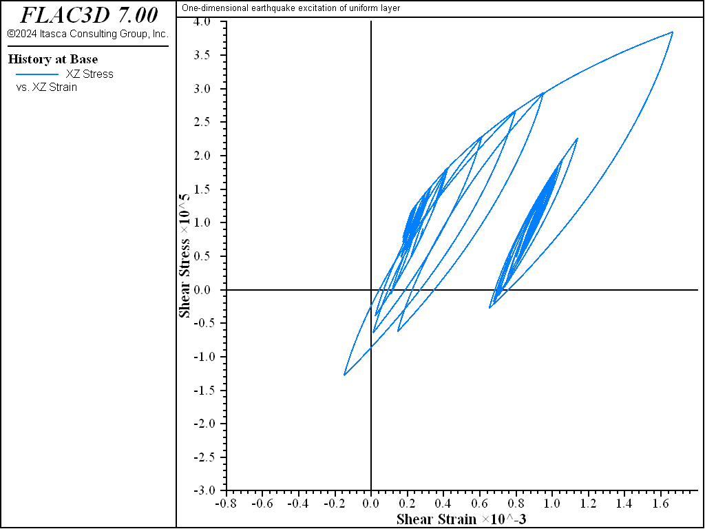
Figure 7: Shear stress vs shear strain for base of the layer. The shear stress is 0.1 MPa and the initial strain is 0.041%, following the static solution.
The approach using a full static solution while hysteretic damping is active in order to obtain a compatible starting state for both stress and strain may be used for more complicated models, such as embankments in which the slope area contains initial shear stresses. One drawback of the approach is that the static solution may involve many diminishing cycles of oscillation as the state of equilibrium is approached. Although these cycles tend to be quite small (and hardly affect the desired stress state), they cause many states to be stored on the memory stack (see Hysteretic Damping Formulation, Implementation and Calibration). These stored states are deleted from the stack early in dynamic loading, but they occupy memory and entail some initial overhead in computer time. It may be possible (in a future version of FLAC3D) to include logic to allow users to flush the stacks at the end of the static initialization, while retaining the latest state of stress-compatible strains for a dynamic simulation with hysteretic damping.
Data Files
EarthquakeExcitation.dat
;---------------------------------------------------------------------
; Script file for Dynamic Problem
; One-dimensional earthquake excitation of uniform layer
;---------------------------------------------------------------------
fish automatic-create off
model new
model large-strain off
model title 'One-dimensional earthquake excitation of uniform layer'
model configure dynamic
; Create zones
zone create brick size 1 1 20
; Assign constitutive model and properties
zone cmodel assign elastic
zone property density 1000 shear 5e8 bulk 10e8
; Boundary conditions
zone gridpoint fix velocity-y
zone gridpoint fix velocity-z
table 'acc' import 'gilroy1.acc'
zone face apply acceleration-x -0.02 table 'acc' range position-z=0
; Histories
model history name='time' dynamic time-total
zone history name='sxz1' stress-xz zoneid = 1
zone history name='exz1' strain-increment-xz zoneid = 1
zone history name='sxz10' stress-xz zoneid = 10
zone history name='exz10' strain-increment-xz zoneid = 10
zone history name='acc00' acceleration-x position (0,0, 0)
zone history name='acc10' acceleration-x position (0,0,10)
zone history name='acc20' acceleration-x position (0,0,20)
; Set damping, cycle to time 25
zone dynamic damping hysteretic default -3.325 0.823
model solve time-total 25
model save 'EarthquakeExcitation'
EarthquakeExcitation-Mod1.dat
;---------------------------------------------------------------------
; Script file for Dynamic Problem
; One-dimensional earthquake excitation of uniform layer
; With shear stress initialize to 0.1 MPa
;---------------------------------------------------------------------
fish automatic-create off
model new
model large-strain off
model title 'One-dimensional earthquake excitation of uniform layer'
model configure dynamic
; Create zones
zone create brick size 1 1 20
; Assign constitutive model and properties
zone cmodel assign elastic
zone property density 1000 shear 5e8 bulk 10e8
; Initial conditions
zone initialize stress-xz 1e5
; Boundary conditions
zone gridpoint fix velocity-y
zone gridpoint fix velocity-z
table 'acc' import 'gilroy1.acc'
zone face apply acceleration-x -0.02 table 'acc' range position-z=0
zone face apply stress-xz 1e5 range union position-z=0 position-z=20
; Histories
model history name='time' dynamic time-total
zone history name='sxz1' stress-xz zoneid = 1
zone history name='exz1' strain-increment-xz zoneid = 1
zone history name='sxz10' stress-xz zoneid = 10
zone history name='exz10' strain-increment-xz zoneid = 10
zone history name='acc00' acceleration-x position (0,0, 0)
zone history name='acc10' acceleration-x position (0,0,10)
zone history name='acc20' acceleration-x position (0,0,20)
; Set damping, cycle to time 25
zone dynamic damping hysteretic default -3.325 0.823
model solve time-total 25
model save 'EarthquakeExcitation-Mod1'
EarthquakeExcitation-Mod2.dat
;---------------------------------------------------------------------
; Script file for Dynamic Problem
; One-dimensional earthquake excitation of uniform layer
;---------------------------------------------------------------------
model new
model large-strain off
model title 'One-dimensional earthquake excitation of uniform layer'
model configure dynamic
; Create zones
zone create brick size 1 1 20
; Assign constitutive models and properties
zone cmodel assign elastic
zone property density 1000 shear 5e8 bulk 10e8
; Boundary conditions
zone gridpoint fix velocity-y
zone gridpoint fix velocity-z
zone face apply stress-xz 1e5 range union position-z=0 position-z 20
; Solve to equilibrium with hysteretic damping active
zone dynamic damping hysteretic default -3.325 0.823
zone dynamic damping local 0.7
model solve
; Reset model
zone gridpoint initialize velocity (0,0,0)
zone dynamic time-total 0
zone dynamic damping local 0.0
; Apply dynamic boundary conditions
table 'acc' import 'gilroy1.acc'
zone face apply acceleration-x -0.02 table 'acc' range position-z=0
; Take some histories
model history name='time' dynamic time-total
zone history name='sxz1' stress-xz zoneid = 1
zone history name='exz1' strain-increment-xz zoneid = 1
zone history name='sxz10' stress-xz zoneid = 10
zone history name='exz10' strain-increment-xz zoneid = 10
zone history name='vel1' acceleration-x position (0,0, 0)
zone history name='vel2' acceleration-x position (0,0,10)
zone history name='vel3' acceleration-x position (0,0,20)
model solve time-total 25
model save 'EarthquakeExcitation-Mod2'
| Was this helpful? ... | FLAC3D © 2019, Itasca | Updated: Feb 25, 2024 |