Embankment Loading on a Cam-Clay Foundation
Problem Statement
Note
To view this project in FLAC3D, use the menu command . Choose “ExampleApplications/EmbankmentLoad” and select “EmbankmentLoad.prj” to load. The project’s main data file is shown at the end of this example.
The response of a saturated soil foundation to loading by a long embankment is studied in this example. The analysis is carried out for a slice of soil foundation of unit thickness normal to the embankment axis. The foundation is 10 meters deep, and the groundwater free surface is at the ground level. The embankment is 8 meters wide. The soil behavior corresponds to a Cam-clay material. The initial stress and pore pressure states correspond to equilibrium under gravity with a ratio of horizontal to vertical effective stress of 6/13. The weight of the embankment is simulated by an applied surcharge and drainage occurs at the soil surface.
The soil has several properties, which are listed in Table 1.
| drained Poisson’s ratio (\(ν\)) | 0.3 |
| soil constant (\(M\)) | 0.888 |
| slope of normal consolidation line (\(λ\)) | 0.161 |
| slope of elastic swelling line (\(κ\)) | 0.062 |
| reference pressure (\(p_1\)) | 100.0 Pa |
| specific volume at reference pressure (\(v_λ\)) | 2.858 |
| porosity | 0.3 |
| dry density (\(ρ\)) | 2 × 10³ kg/m3 |
The clay is lightly over-consolidated, and the initial value of the cap pressure, \(p_c\), is equal to 1.6 × 10⁵ Pa in the example. (Note that for a normally consolidated soil, the value for \(p_c\) is equal to 1.579 × 10⁵ Pa at the base of the clay layer, where \(p\) = 8.33 × 10⁴ Pa and \(q\) = 7.0 × 10⁴ Pa.) The drained Poisson’s ratio of the material is assumed to remain constant during the simulation.
The foundation has a permeability, \(k\), of 10-12 (m/s)/(Pa/m). The soil moduli are functions of the mean effective pressure and the soil-specific volume, quantities that vary in space and evolve during the simulation. The average value of \(K + 4/3 G\), however, stays of the order of 106 Pa, or two orders of magnitude lower than the water bulk modulus (\(K_w\) is 2 × 10⁸ Pa). The diffusivity, \(c\), is thus controlled by the soil material in this example. Its magnitude can be estimated from the formula \(c = k(K + 4/3 G)\), and is of the order of 10-6 m2/s. The time scale for the diffusion process can be estimated using \(t_c\) = \(L\)2/\(c\), where \(L\) is the model height. Using \(L\) = 10 m, we have that \(t_c\) is of the order of three years. Compared to that time, construction of the embankment may be assumed to occur instantaneously. An undrained analysis is first conducted to evaluate the foundation settlement in the short-term after building of the embankment; the long-term response is then monitored after allowing drainage from the soil surface.
Modeling Procedure
The model, represented in Figure 1, takes advantage of half-symmetry. The size is 20 meters wide and 10 meters deep. Note that the width of the model is not necessarily large enough to accurately represent an extensive soil layer; the model is intended for illustrative purposes only. The mechanical boundary conditions correspond to roller boundaries on both sides of the plane of analysis (\(y\)-direction), roller boundaries along the symmetry line and the far boundary of the model (\(x\)-direction), and to fixed displacements in the \(x\)-, \(y\)-, and \(z\)-direction at the model base. The maximum bulk modulus of the clay (bulk-maximum) is set to 5 × 10⁶ Pa, a value that is approximately twice the initial value of the actual bulk modulus (bulk) at the bottom of the clay layer.
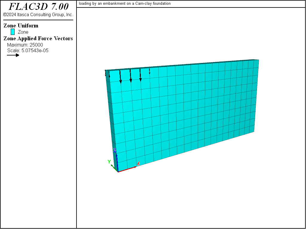
Figure 1: Model geometry.
The first stage of the simulation corresponds to the short time response of the system in which no flow is assumed to take place.
The command model fluid active off is specified.
Loading by the embankment is simulated by progressive application of a pressure of 50 kPa on a 4 meter section of the model top boundary
(to reproduce proportional loading conditions).
Once the full load is attained,
the model is cycled to equilibrium.
During this stage, pore pressures develop as a result of volumetric deformations, but do not dissipate.
In the second stage, fluid flow is allowed to develop by issuing the command model fluid active on.
Water then drains through the top of the model where the pore pressure is fixed at zero,
and additional settlement takes place under the embankment.
The model solve fluid time-total command, used to perform the coupled simulation,
requires parameters that determine the accuracy of the solution.
These parameters may need to be adjusted if different properties or model conditions are used.
Refer to Coupled Flow and Mechanical Calculations for a discussion on these topics.
Stresses, pore pressures, and vertical displacements are monitored during the calculation.
The data file for this problem is listed in the end of this page.
Results and Discussion
Displacement vectors, vertical displacement contours, and the pore pressure distribution at the end of the undrained and drained numerical simulations are presented in Figure 2 to Figure 7. The vertical displacement histories in Figure 8, recorded at four monitoring points, indicate that the maximum settlement under the embankment increases from approximately 0.14 m to 0.19 m as a result of drainage. Note that the displacement vectors in Figure 3 and vertical displacement contours in Figure 5 correspond to the combined undrained and drained displacements.
In Figure 9, the graph of pore pressure evolution at two monitoring points confirms that a steady-state flow has been reached by the end of the drained simulation.
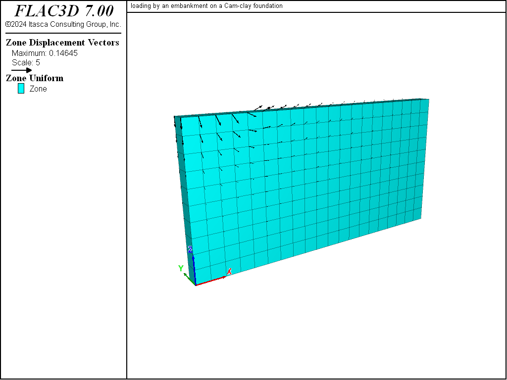
Figure 2: Displacement vectors—undrained response.
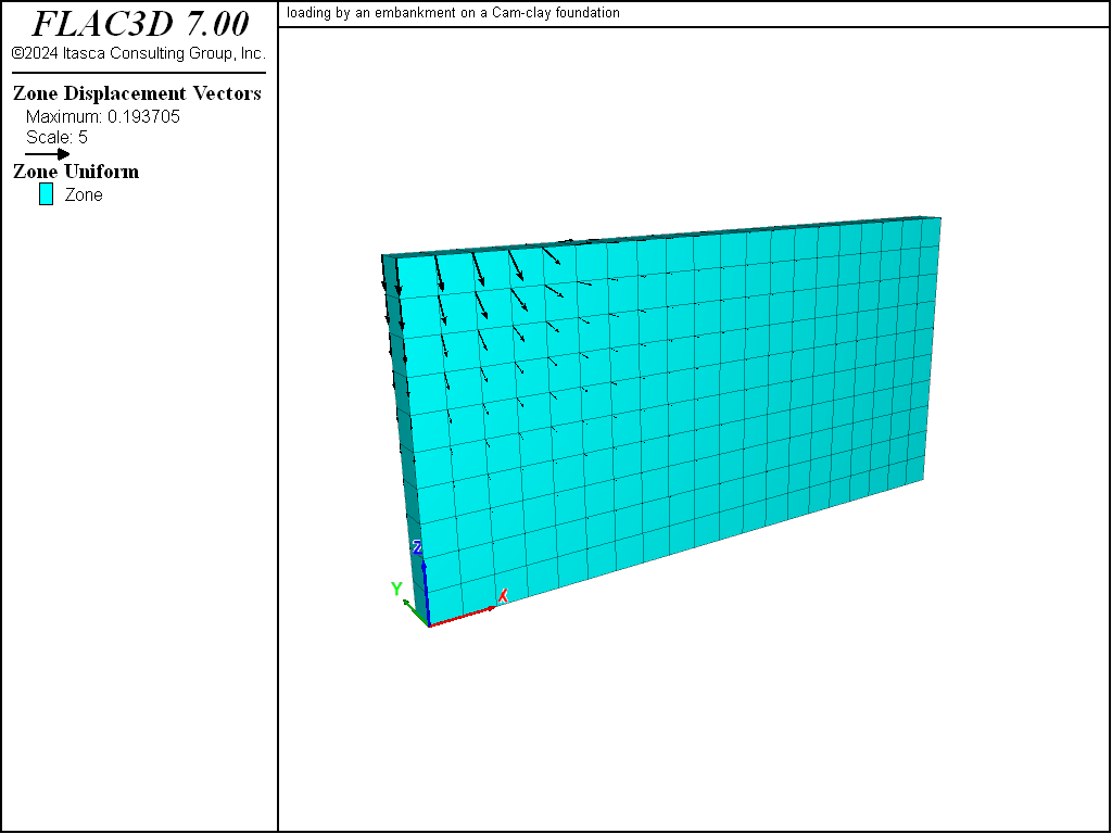
Figure 3: Displacement vectors—end of drained simulation.
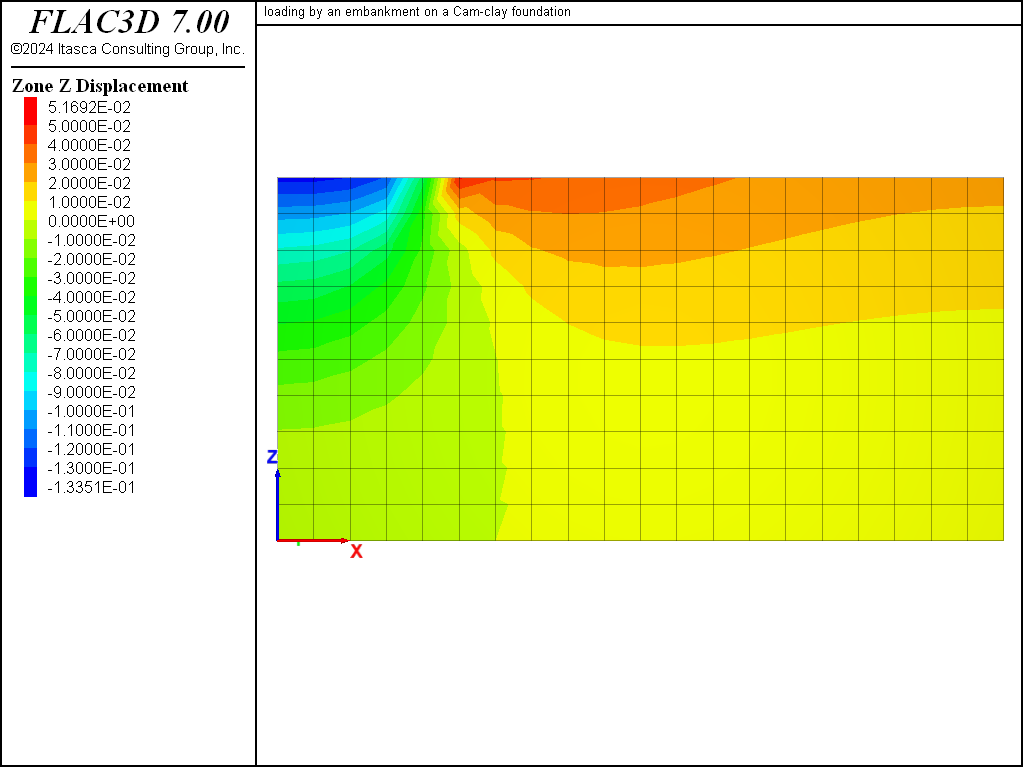
Figure 4: Vertical displacement contours—undrained response.
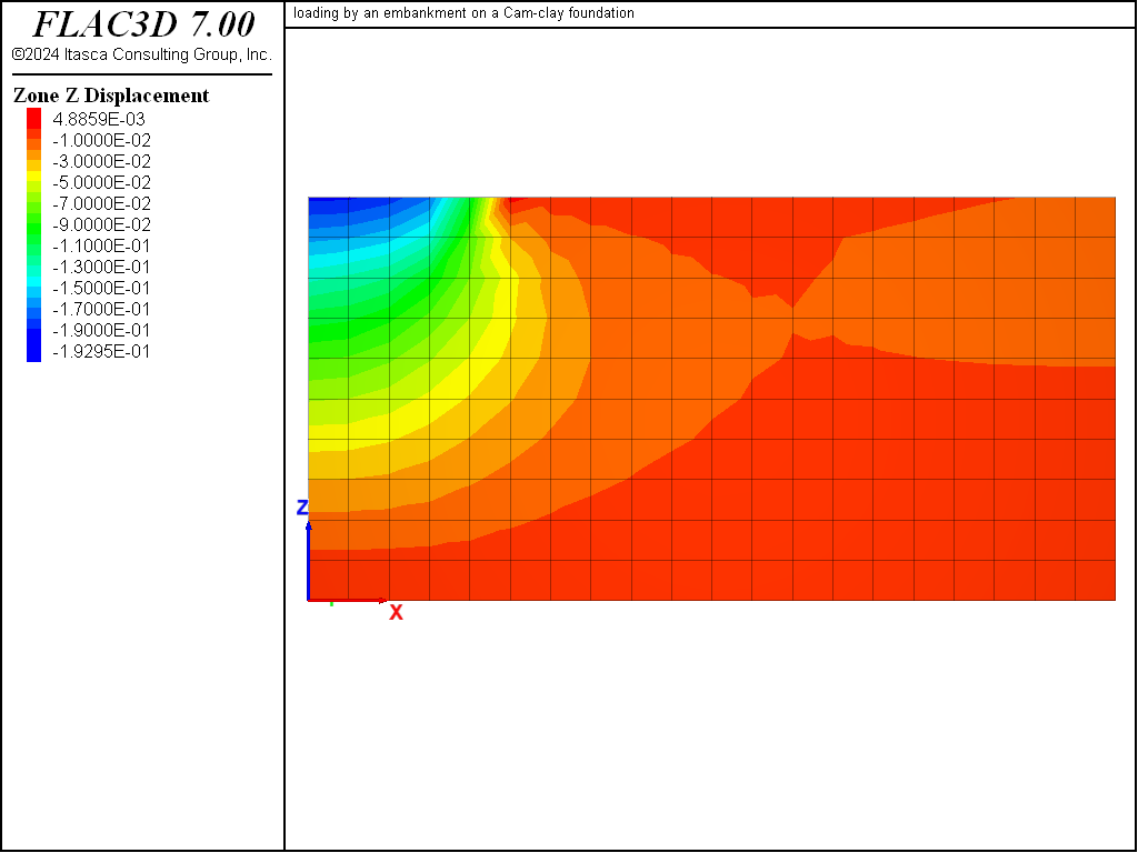
Figure 5: Vertical displacement contours—end of drained simulation.
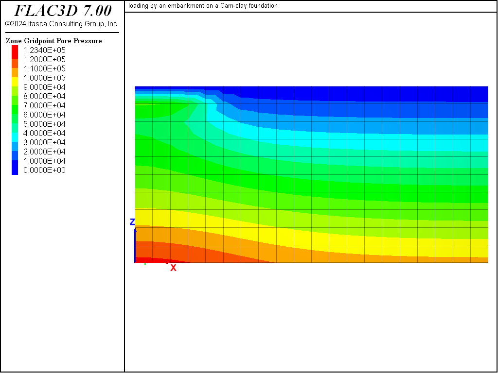
Figure 6: Pore pressure contours—undrained response.
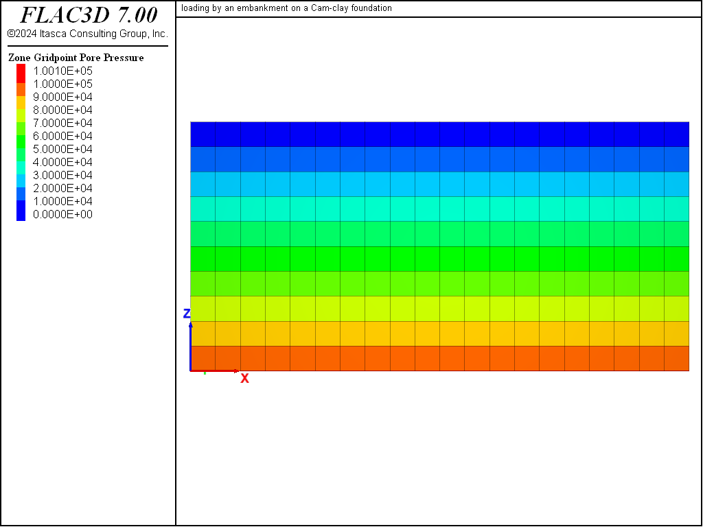
Figure 7: Pore pressure contours—drained response.
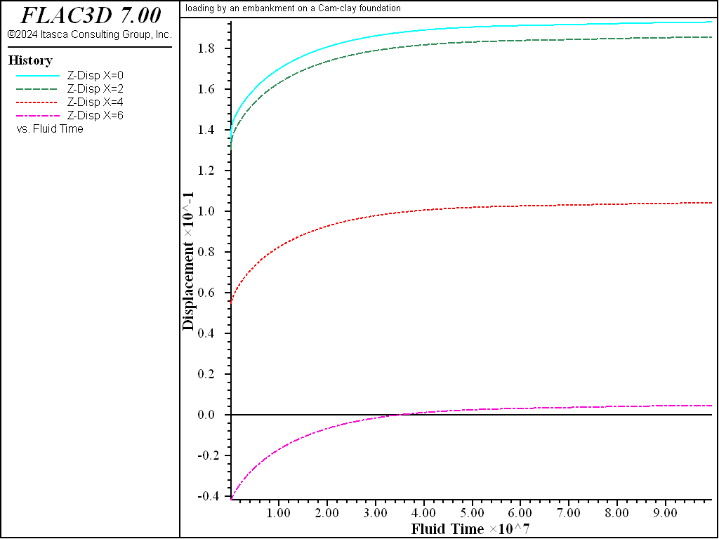
Figure 8: Vertical displacement histories—drained response.
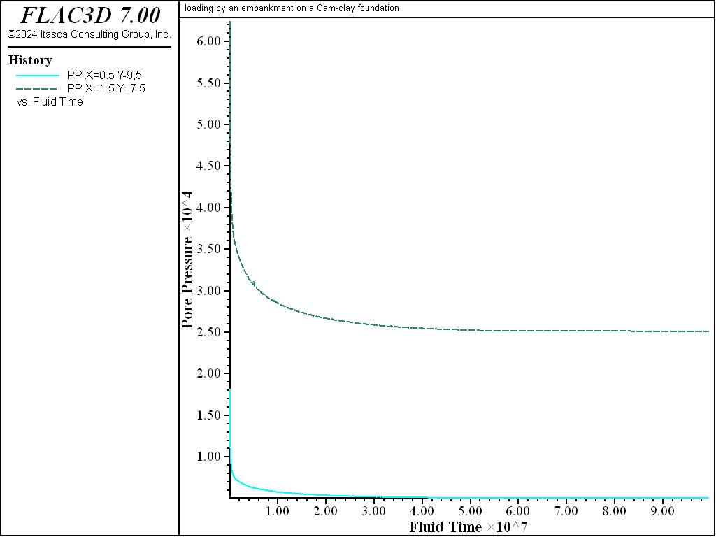
Figure 9: Pore pressure histories—drained response.
Data File
EmbankmentLoad.dat
;-----------------------------------------------------------
; Loading by an embankment on a Cam-clay foundation
;-----------------------------------------------------------
model new
model large-strain off
fish automatic-create off
model title "loading by an embankment on a Cam-clay foundation"
model config fluid
; -- Create zone geometry
zone create brick point 0 (0,0,0) point 1 (20,0,0) point 2 (0,1,0) ...
                  point 3 (0,0,10) ...
                  size 20 1 10
zone face skin ; Name model boundaries
; --- mechanical model and properties ---
zone cmodel assign modified-cam-clay
zone property poisson .3 bulk-maximum 5e6 density 2000
zone property ratio-critical-state 0.888 lambda 0.161 kappa 0.062
zone property pressure-preconsolidation 160e3 pressure-reference 1e3 ...
              specific-volume-reference 2.858
; -- fluid model and properties
zone fluid cmodel assign isotropic
zone fluid biot off
zone fluid property permeability 1e-12 porosity .3
zone gridpoint initialize fluid-modulus 2e8
zone gridpoint initialize fluid-tension -1e20
zone initialize fluid-density 1e3
; --- initial conditions ---
model gravity 10
zone gridpoint initialize saturation 1
zone initialize-stresses ratio 0.7
zone gridpoint initialize pore-pressure 1e5 gradient (0,0,-1e4)
program call 'pressure-effective' suppress ; FISH to initialize the CamClay
                                   ; property of mean effective stress
[pressure_effective]
; --- boundary conditions ---
zone face apply velocity-normal 0 range group 'East' or 'West'
zone face apply velocity-normal 0 range group 'North' or 'South'
zone face apply velocity (0,0,0) range group 'Bottom'
zone face apply pore-pressure 0 range group 'Top'
zone face apply stress-normal=-5e4 servo ramp ratio local ...
          range position-x 0 4 group 'Top'
; --- settings ---
model mechanical active on
model fluid active off
; --- histories ---
history interval 100
zone history name 'z0' displacement-z position (0,0,10)
zone history name 'z2' displacement-z position (2,0,10)
zone history name 'z4' displacement-z position (4,0,10)
zone history name 'z6' displacement-z position (6,0,10)
zone history name 'pp1' pore-pressure position (0.5,0.5,9.5)
zone history name 'pp2' pore-pressure position (1.5,0.5,7.5)
; --- undrained response ---
model solve ratio-local 1e-4
model save 'undrained'
; --- drained response ---
model fluid active on
model history name 'time' fluid time-total
model fluid substep 100
model mechanical substep 10
model mechanical slave
model solve time-total 1e5 or mechanical ratio 5e-5
model mechanical substep 50
model solve time-total 1.e8 or mechanical ratio 5e-5
model save 'drained'
| Was this helpful? ... | FLAC3D © 2019, Itasca | Updated: Feb 25, 2024 |