Conduction in a Plane Sheet
Note
To view this project in FLAC3D, use the menu command . Choose “Thermal/PlaneSheetConduction” and select “PlaneSheetConduction.prj” to load. The project’s main data files are shown at the end of this example.
A plane sheet of thickness \(L\) = 1 m is initially at a constant temperature of 0°C. One side of the sheet is exposed to a constant temperature of 100°C, while the other side is kept at 0°C. The sheet eventually reaches an equilibrium state at a constant heat flux and unchanging temperature distribution.
The analytical solution to this problem for the transient temperature distribution is given by Crank (1975):
where:
\(T_1\) is the fixed temperature at \(z\) = 0 of the sheet;
\(T_2\) is the fixed temperature at \(z\) = L of the sheet;
\(L\) is the width of the sheet;
\(t\) is time;
\(z\) is distance across the sheet;
\(f(z)\) is the initial temperature distribution function in the range of \(0 < z < L\); and
\(\kappa\) is equal to \(k/({\rho}C_p)\), where \(k\) is the thermal conductivity, \(\rho\) is the density, and \(C_p\) is the specific heat.
Particularly for \(f(z) = T_2\) (the case in this example), the solution becomes
The thermal conductivity for this example is 1.6 W/m °C, the specific heat is 0.2 J/kg °C, the mass density of the material is 1000 kg/m3, and the temperature, \(T\), is 100°C.
The analytical solution is programmed as a FISH function for direct comparison to the numerical results at selected thermal times. The analytical and numerical temperature results for these times are stored in tables.
In the FLAC3D model, the sheet is defined as a column of 25 zones. A constant temperature boundary of 100°C is applied at the face located at \(z\) = 0, and a constant temperature boundary of 0 °C is applied at the face located at \(z\) = 1. The model grid is shown in Figure 1:
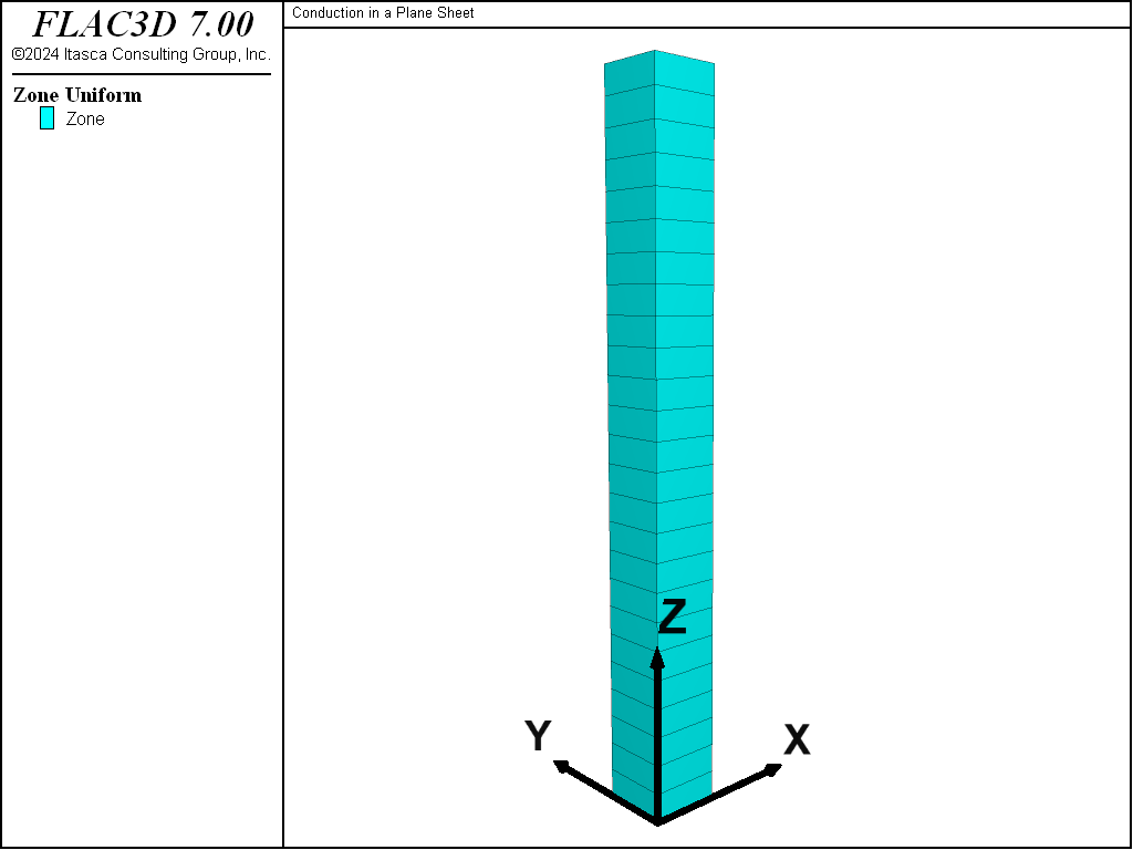
Figure 1: FLAC3D grid for conduction in a plane sheet.
This example contains solutions solved by FLAC3D using both explicit and implicit formulations. The comparison of analytical and numerical temperatures at three thermal times for the explicit solution is shown in Figure 2, and that for the implicit solution in Figure 3. Normalized temperature (\((T(z,t)-T_2)/(T_1-T_2)\)) is plotted versus normalized distance (\(z/L\)) in the two figures, where Tables 2, 4, and 6 contain the analytical solution for temperatures, and Tables 1, 3, and 5 contain the FLAC3D solutions. The three thermal times are 2, 12, and 72 seconds for both the explicit and implicit solutions. The solution has reached the equilibrium thermal state by the last time in each case. For both solution formulations, the difference between analytical and numerical temperatures at steady state is less than 0.1%. Note that for the explicit solution, the timestep is approximately 0.07 seconds, while for the implicit solution, the timestep is set to 0.1 seconds.
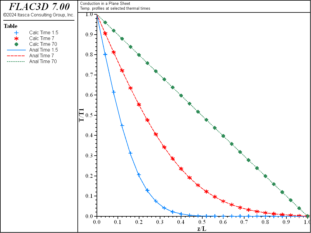
Figure 2: Comparison of temperatures for the explicit-solution algorithm (analytical values = crosses; numerical values = lines).

Figure 3: Comparison of temperatures for the implicit-solution algorithm (analytical values = crosses; numerical values = lines).
Reference
Crank, J. The Mathematics of Diffusion, 2nd Ed. Oxford: Oxford University Press (1975).
Data File
; Thermal conduction in a plane sheet
; Compares explicit and implicit methods
model new
model large-strain off
fish automatic-create off
model title 'Conduction in a Plane Sheet'
model configure thermal

; --- main computation ---
zone create brick size 1 1 25 point 1 (0.1,0,0) ...
                              point 2 (0,0.1,0) point 3 (0,0,1)
; -- thermal model
zone thermal cmodel isotropic
zone thermal property conductivity 1.6 specific-heat 0.2
zone initialize density 1000
zone face apply temperature 100. range position-z 0.0
zone face apply temperature   0. range position-z 1.0
; settings
model mechanical active off
model thermal active on
model save 'psheet-ini'

; -- explicit method
; test
model solve time-total 1.5
model save 'psheet-exp-015'
model solve time-total 7
model save 'psheet-exp-070'
model solve time-total 70
model save 'psheet-exp-700'

; -- implicit method
model restore 'psheet-ini'
; test - start with explicit method
model solve time-total 1.5
model save 'psheet-exp-015'
; - then switch to implicit
zone thermal implicit on
model thermal timestep fix 1.e-1
model solve time-total 7
model save 'psheet-imp-070'
model solve time-total 70
model save 'psheet-imp-700'

program return
| Was this helpful? ... | FLAC3D © 2019, Itasca | Updated: Feb 25, 2024 |