Measured Quantities
In this topic, each of the measurement quantities available in the measure logic is defined, and the assumptions and approximations employed in their computation are described.
These quantities are:
Coordination Number | Porosity | Stress | Strain Rate | Size Distribution
Coordination Number
The coordination number, \(C_n\), is defined as the average number of active contacts per body (where a body can be either a ball or a clump), and is computed as
where the summation is taken over the \(N_b\) bodies with centroids in the measurement region, and \(n_c^{(b)}\) is the number of active contacts of body \(b\). Note that contact activity depends on the contact model installed at the contact (refer to the “Contact Models” section for further details).
Porosity
The porosity, \(n\), is defined as the ratio of total void volume, \(V^{void}\), within the measurement region to measurement-region volume, \(V^{reg}\):
where \(V^{mat}\) is the volume of material in the measurement region. \(V^{mat}\) is approximated by (see the figure below)
where \(N_b\) is the number of bodies that lie fully within the measurement region, \(V^{(b)}\) is the volume of body \(b\), \(\bar{N}_b\) is the number of bodies that intersect the measurement region, \(\bar{V}^{(b)}\) is the intersection volume between body \(b\) and the measurement region, \(N_c\) is the number of contacts that lie in the measurement region, and \(V^{(c)}\) is the overlap volume of the two bodies at contact \(c\). Note that a clump is considered to lie fully within a measurement region if each of its constituent pebble does.
The intersection volume between a ball with center at position \(\mathbf{X_1}\) and radius \(R_1\) and a measurement region with center \(\mathbf{X_2}\) and radius \(R_2\) is given by
where:
The intersection volume between a clump and a measurement region is approximated via a voxelization approach, as discussed in
the measure create command description.
The overlap volume of two bodies at contact \(c\) is computed using Equations (4) and (5), where the subscripts denote the two pieces (ball or pebble) in contact.
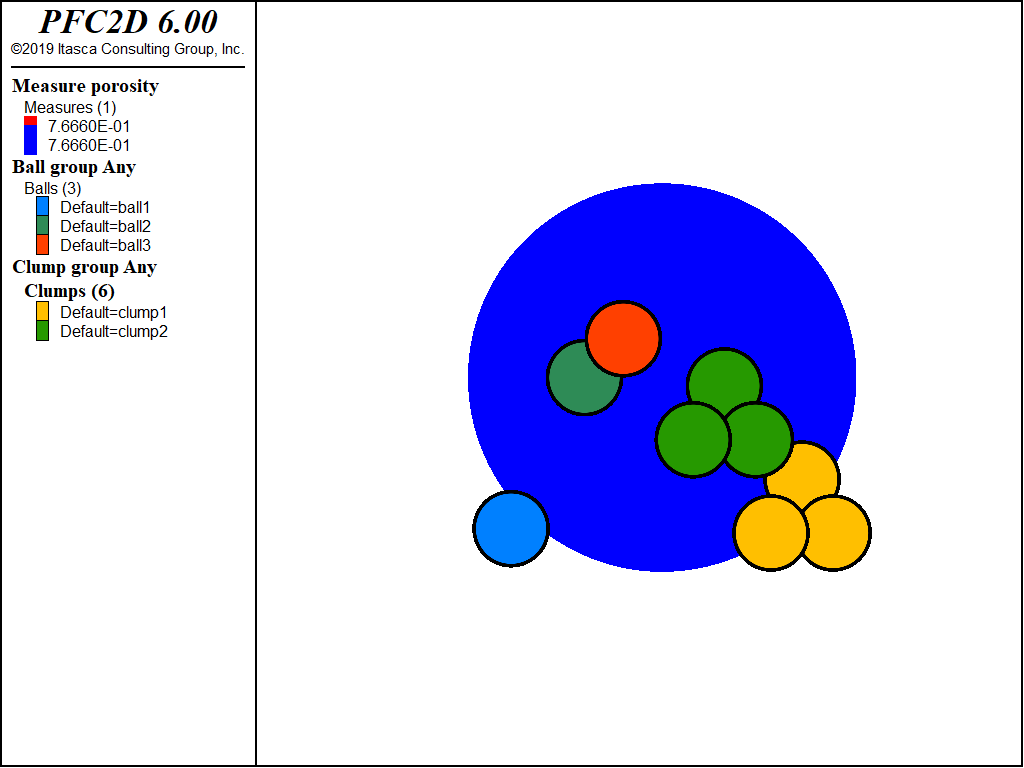
Figure 1: Porosity computation for a system with 3 balls and 2 clumps. Ball 1 and clump 1 intersect the measurement region, and only their respective intersection volumes contribute to the porosity computation. Ball 2, ball 3, and clump 2 lie fully inside the measurement region, and therefore contribute their entire volume. Balls 2 and 3 and clumps 1 and 2 are in contact within the measurement region: respective contact overlap volumes are subtracted from the total volume of material used in Equation (2).
Stress
Stress is a continuum quantity and, therefore, does not exist at each point in a particle assembly, because the medium is discrete (see figure below). In the discrete PFC model, contact forces and particle displacements are computed. These quantities are useful when studying the material behavior on a microscale, but they cannot be transferred directly to a continuum model. Averaging procedures are necessary to make the step from the microscale to a continuum. The average stress \(\bar\sigma_{ij}\) in a measurement region of volume \(V\) is computed as ([Christoffersen1981]):
where \(N_c\) is the number of contacts that lie in the measurement region or on its boundary, \(\mathbf{F^{(c)}}\) is the the contact force vector, \(\mathbf{L^{(c)}}\) is the branch vector joining the centroids of the two bodies in contact, \(\otimes\) denotes outer product, and compressive stress is negative by convention. Note that the underlying assumptions behind the formula above are based on a static analysis. Alternative computations may be desired for dynamic situations (for example, see [Fortin2003]).
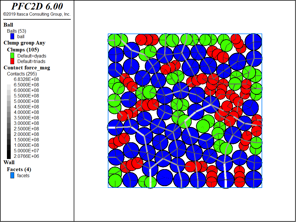
Figure 2: Typical particulate material consisting of circular/spherical particles (2D/3D) and two- and three-particle clumps, along with contact forces. The 2D case is shown here for clarity.
Strain Rate
The procedure employed to measure local strain rate within a particle assembly differs from that used to measure local stress. In the determination of local stress, the average stress within a volume of material is expressed directly in terms of the discrete contact forces, because the forces in the voids are zero. It is not correct, however, to use the velocities in a similar way to express the average strain rate, because the velocities in the voids are nonzero. Instead of assuming a form for the velocity field in the voids, a strain-rate tensor, based on a best-fit procedure that minimizes the error between the predicted and measured velocities of all balls with centroids contained within the measurement region, is determined.
Before describing the least-squares procedure, the relation between the strain and strain rate will be reviewed and the corresponding terms defined.
The relation between the displacements \(u_i\) at two neighboring points is given by the displacement gradient tensor, \(\alpha_{ij}\). Let the particles \(P\) and \(P'\) be located instantaneously at \(x_i\) and \(x_i + dx_i\), respectively. The difference in displacement between these two points is
The displacement gradient tensor can be decomposed into a symmetric tensor and an antisymmetric tensor as
where:
In a similar fashion, the relation between the velocities, \(v_i\), at two neighboring points is given by the velocity gradient tensor, \(\dot\alpha_{ij}\). (The velocity field is related to the displacement field by \(u_i = v_i dt\), in which \(v_i\) is the velocity and \(dt\) is an infinitesimal interval of time.) Let the particles \(P\) and \(P'\) be located instantaneously at \(x_i\) and \(x_i + dx_i\), respectively. The difference in velocity between these two points is
The velocity-gradient tensor can be decomposed into a symmetric tensor and an antisymmetric tensor as
where:
In PFC, the velocity-gradient tensor, \(\dot\alpha_{ij}\), is referred to as the strain-rate tensor. \(\dot\alpha_{ij}\) is computed using the following least-squares procedure.
The strain-rate tensor computed for a given measurement region represents the best fit to the \(N_p\) measured relative velocity values, \(\tilde V_i^{(p)}\), of the particles with centroids contained within the measureword. The mean velocity and position of the \(N_p\) particles is given by
where \(V_i^{(p)}\) and \(x_i^{(p)}\) are the translational velocity and centroid location, respectively, of particle \((p)\). The measured relative velocity values are given by
For a given \(\dot\alpha_{ij}\), the predicted relative velocity values, \(\tilde v_i^{(p)}\), can be written using Equation (10) as
where
A measure of the error in these predicted values is given by
where \(z\) is the sum of the squares of the deviations between predicted and measured velocities. The condition for minimum \(z\) is that
Substituting Equation (15) into Equation (17) and differentiating, the following set of nine equations is obtained:
These nine equations are solved by performing a single LU-decomposition upon the 3 × 3 coefficient matrix, and performing three back-substitutions for the three different right-hand sides obtained by setting \(i\) = 1, 2, and then 3. In this way, all nine components of the strain-rate tensor are obtained.
Size Distribution
The cumulative volume percentage of bodies that lie fully in or intersect a measurement region can be computed and
exported into a table using the measure dump command. All bodies whose centroids fall within the measurement region
are binned based on the {area in 2D; volume in 3D} equivalent {circle in 2D; sphere in 3D} diameters, and on the bins
defined with the measure create or measure modify command. The data can also be exported into a FISH
array using the measure.size intrinsic.
References
| [Christoffersen1981] | Christoffersen, J., M. M. Mehrabadi and S. Nemat-Nasser. “A micromechanical description of granular material behavior,” J. Appl. Mech., 48, 339-344, 1981. |
| [Fortin2003] | Fortin, J., O. Millet and G. de Saxcé. “Construction of an averaged stress tensor for granular medium,” European Journal of Mechanics A/Solids, 22, 567-582, 2003. |
| Was this helpful? ... | FLAC3D © 2019, Itasca | Updated: Feb 25, 2024 |