Contact Resolution
Contact resolution occurs when a new contact is detected during the cycle sequence, prior to force-displacement calculations. During contact resolution, the contact state variables (see table) are updated. These variables are defined, and the procedure by which they are computed is described here.
The contact shown in Figure 1 has been created between the pieces of two bodies. Each contact has two ends, end1 and end2, with the associated pieces and bodies labeled 1 and 2. The bodies are rigid; therefore, the motion of body \((b)\) is described by its rotational velocity \(( \pmb{ω}^{(b)} )\) and the translational velocity \(( \dot{\mathbf{x}}^{(b)} )\) of its centroid \(( \mathbf{x}^{(b)} )\).
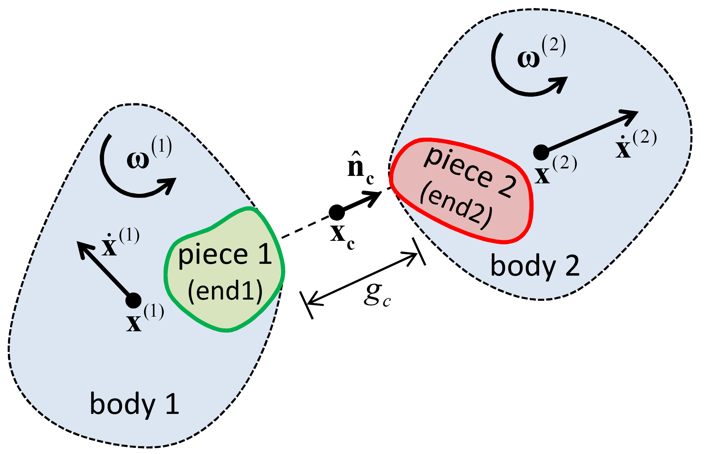
Figure 1: A contact between the pieces of two bodies.
The first contact state variables to be updated are: the effective inertial mass of the contact \(( m_c )\); the location \(( \mathbf{ x_c } )\), normal direction \(( \hat{\mathbf{n}}_\mathbf{c} )\) and coordinate system \(( nst )\) of the contact plane; and the contact gap \(( g_c )\), which is the minimal signed distance separating the piece surfaces. The contact mass is given by
where \(m^{(b)}\) is the mass of body \((b)\). Computation of the location, normal direction and gap depends on the surface geometry of the two contacting pieces in the vicinity of the contact (and is described below in the “Contact Plane” section).
After the above quantities have been updated, the contact model is responsible for updating the activity state of the contact, given the updated contact gap. The exact criterion used to determine contact activity is specific to the implementation of each contact model. If the contact was not found to be active, then an additional check is performed to assess whether, given the current conditions, it could become active in the near future. Both active and could-be-active contacts participate in the timestep estimation procedure. If the contact is found active, then the variables defining the relative motion of the piece surfaces are computed (as described in “Relative Motion at a Contact” section).
The kinematic information is described in the next two sections, which define the contact plane and describe the relative motion of the piece surfaces at a contact. All contact types are described without loss of generality in terms of the two combinations of ball-ball and ball-facet, because balls and pebbles have the same shape. The ball-ball contact types include ball-ball, ball-pebble, and pebble-pebble; the ball-facet contact types include ball-facet and pebble-facet.
| Property | Description |
|---|---|
| \(m_c\) | effective inertial mass |
| Contact plane: | |
| \(\mathbf{ x_c }\) | contact-plane location |
| \(\hat{\mathbf{n}}_\mathbf{c}\) | contact-plane normal direction |
| \(\hat{\mathbf{s}}_\mathbf{c}\) | contact-plane coordinate system (\(s\) axis) (2D model: \(\;\hat{\mathbf{s}}_\mathbf{c} \equiv -\hat{\mathbf{k}}\)) |
| \(\hat{\mathbf{t}}_\mathbf{c}\) | contact-plane coordinate system (\(t\) axis) |
| \(g_c\) | contact gap |
| Relative motion: | |
| \(\dot{\pmb{δ}}\) | relative translational velocity |
| \(\dot{\pmb{θ}}\) | relative rotational velocity |
| \(\Delta\delta_n\) | relative normal-displacement increment |
| \(\Delta\pmb{δ}_\mathbf{s}\) | relative shear-displacement increment \((\Delta\delta_{ss},\Delta\delta_{st})\) (2D model: \(\Delta\delta_{ss}\equiv 0\)) |
| \(\Delta\theta_t\) | relative twist-rotation increment (2D model: \(\Delta \theta _{t} \equiv 0\)) |
| \(\Delta\pmb{θ}_\mathbf{b}\) | relative bend-rotation increment \((\Delta\theta_{bs},\Delta\theta_{bt})\) (2D model: \(\Delta \theta _{bk} =-\Delta \theta _{bs},\Delta \theta _{bt} \equiv 0\)) |
Contact Plane
A contact provides an interface between two pieces (see Figure 2). The interface consists of a contact plane with location \(( \mathbf{ x_c } )\), normal direction \(( \hat{\mathbf{n}}_\mathbf{c} )\), and coordinate system \(( nst )\). The contact plane is centered within the interaction volume (either gap or overlap) of the two pieces, oriented tangential to the two pieces and rotated to ensure that relative motion of the piece surfaces at the contact location remains symmetric w.r.t. the contact plane.
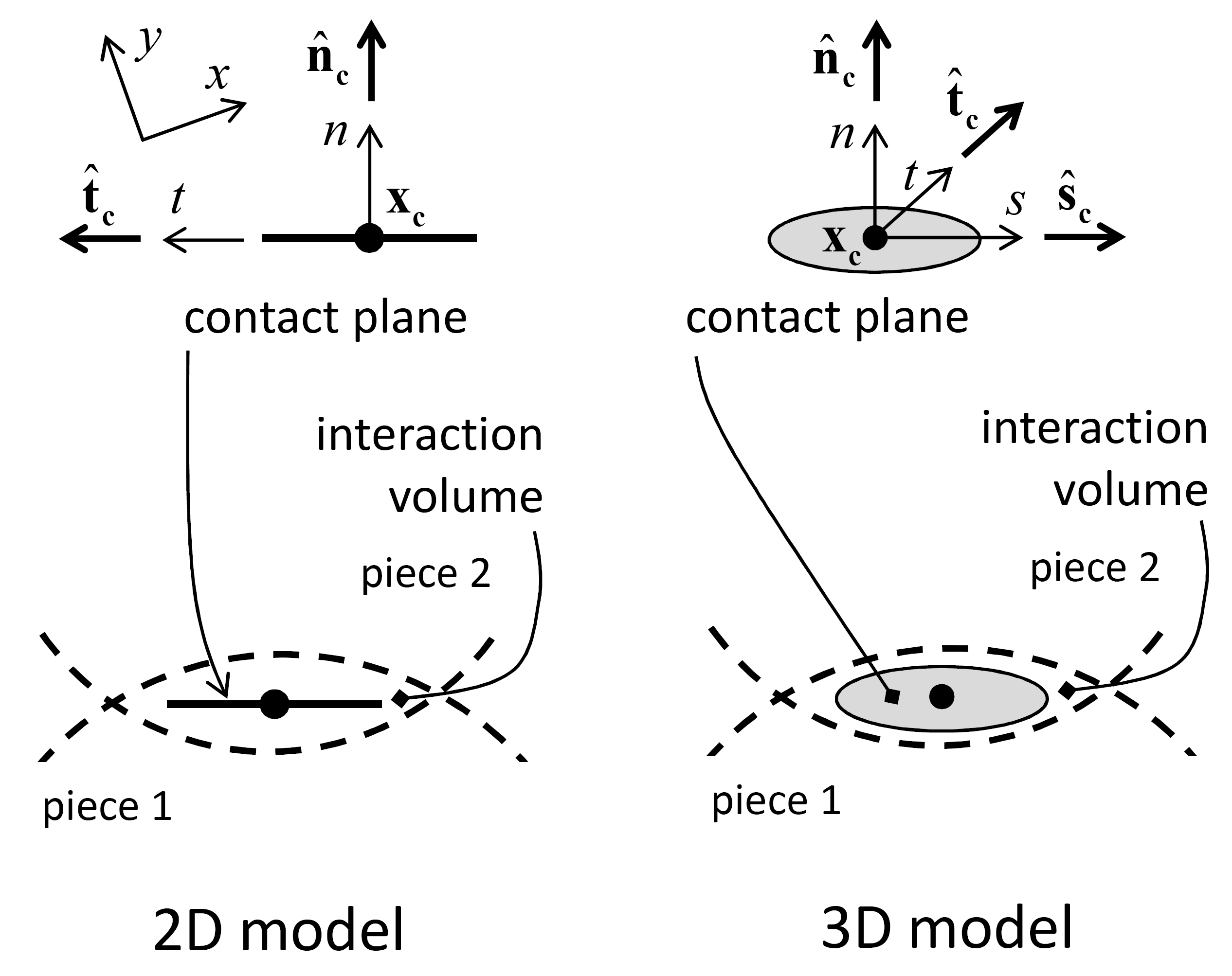
Figure 2: The contact plane coordinate systems for the 2D and 3D models.
The contact plane is centered within the interaction volume of the two pieces, directed from piece 1 to piece 2 and oriented tangential to piece 1. The location \(( \mathbf{ x_c } )\) and normal direction \(( \hat{\mathbf{n}}_\mathbf{c} )\) of the contact plane are given by (see Figure 3):
where \(\mathbf{x}^{(b)}\) and \(R^{(b)}\) are the center and radius, respectively, of ball \((b)\); \(\mathbf{x_f}\) is the point on the wall facet that is closest to \(\mathbf{x}^{(1)}\); \(\mathbf{x_w}\) is the wall center of rotation and \(g_c\) is the contact gap. The contact gap is the minimal signed distance separating the piece surfaces such that the gap is negative if the surfaces overlap.
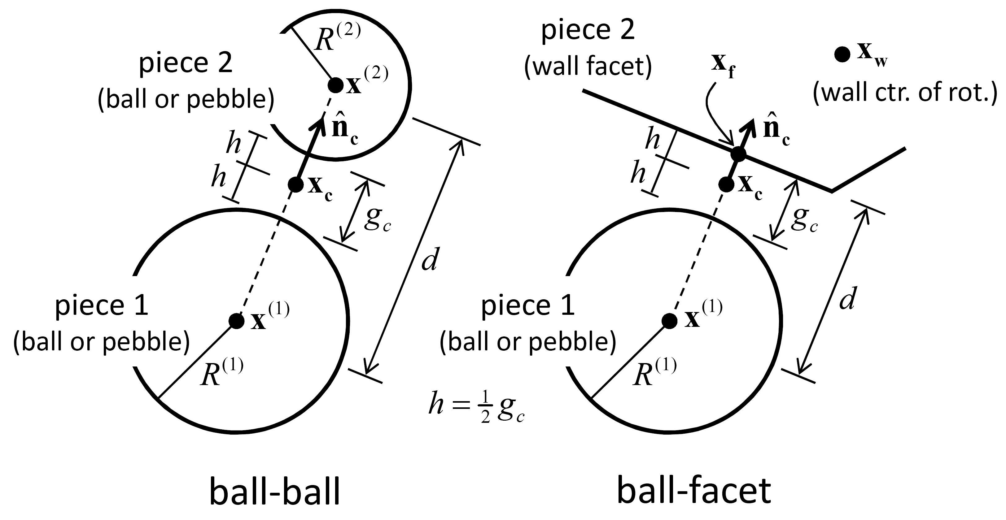
Figure 3: The contact plane location and normal direction for the two fundamental contact types: ball-ball and ball-facet.
The contact plane coordinate system \(( nst )\) is oriented such that \(n\) coincides with the contact normal direction while \(s\) and \(t\) are orthogonal coordinates on the plane and \(\hat{\mathbf{n}}_\mathbf{c} = \hat{\mathbf{s}}_\mathbf{c} \times \hat{\mathbf{t}}_\mathbf{c}\). The contact plane coordinate system is translated and rotated to ensure that relative motion of the piece surfaces at the contact location remains symmetric w.r.t. the contact plane (as shown in Figure 7 and Figure 8). The translation updates the location and normal direction via Equation (2). For the 2D model, the following constraints make the rotation implicit:
The contact location and normal direction lie in the \(xy\) plane such that
(3)\[\begin{split}\begin{array}{l} {\mathbf{x_c} =\mathbf{x_{c}} (x,y,z)=x_{cx} {\kern 1pt} \hat{\mathbf{i}}+x_{cy} {\kern 1pt} \hat{\mathbf{j}}+x_{cz} {\kern 1pt} \hat{\mathbf{k}}\; \; \left(x_{cz} \equiv 0\right)} \\[3mm] {\hat{\mathbf{n}}_\mathbf{c} =\hat{\mathbf{n}}_\mathbf{c} (x,y,z)=n_{cx} {\kern 1pt} \hat{\mathbf{i}}+n_{cy} {\kern 1pt} \hat{\mathbf{j}}+n_{cz} {\kern 1pt} \hat{\mathbf{k}}\; \; \left(n_{cz} \equiv 0\right).} \end{array}\end{split}\]The \(nt\) axis lies in the \(xy\) plane such that
(4)\[ \hat{\mathbf{t}}_\mathbf{c} = \hat{\mathbf{k}} \times \hat{\mathbf{n}}_\mathbf{c}.\]
For the 3D model, the \(s\)-axis is aligned initially with the projection of the global \(x\) or \(y\) direction, respectively, onto the contact plane (whichever is not parallel with \(\hat{\mathbf{n}}_\mathbf{c}\)), and then the rotation updates the \(s\)-axis orientation:
where the first rotation (to give \(\mathbf{s}_{1}\)) is about the line common to the old and new planes, and the second rotation (to give \(\mathbf{s}_{2}\)) is about the new normal direction; the star (\(*\)) denotes the value at the end of the previous timestep; \(\pmb{ω} ^{(p)}\) is the rotational velocity of piece \((p)\); and \(\tilde{\pmb{ω} }\) is the average rotational velocity of the two pieces about the new normal direction. See Figure 4 and note that the vector \(\mathbf{S}\) rotates with the plane (as if it were marked onto the plane).
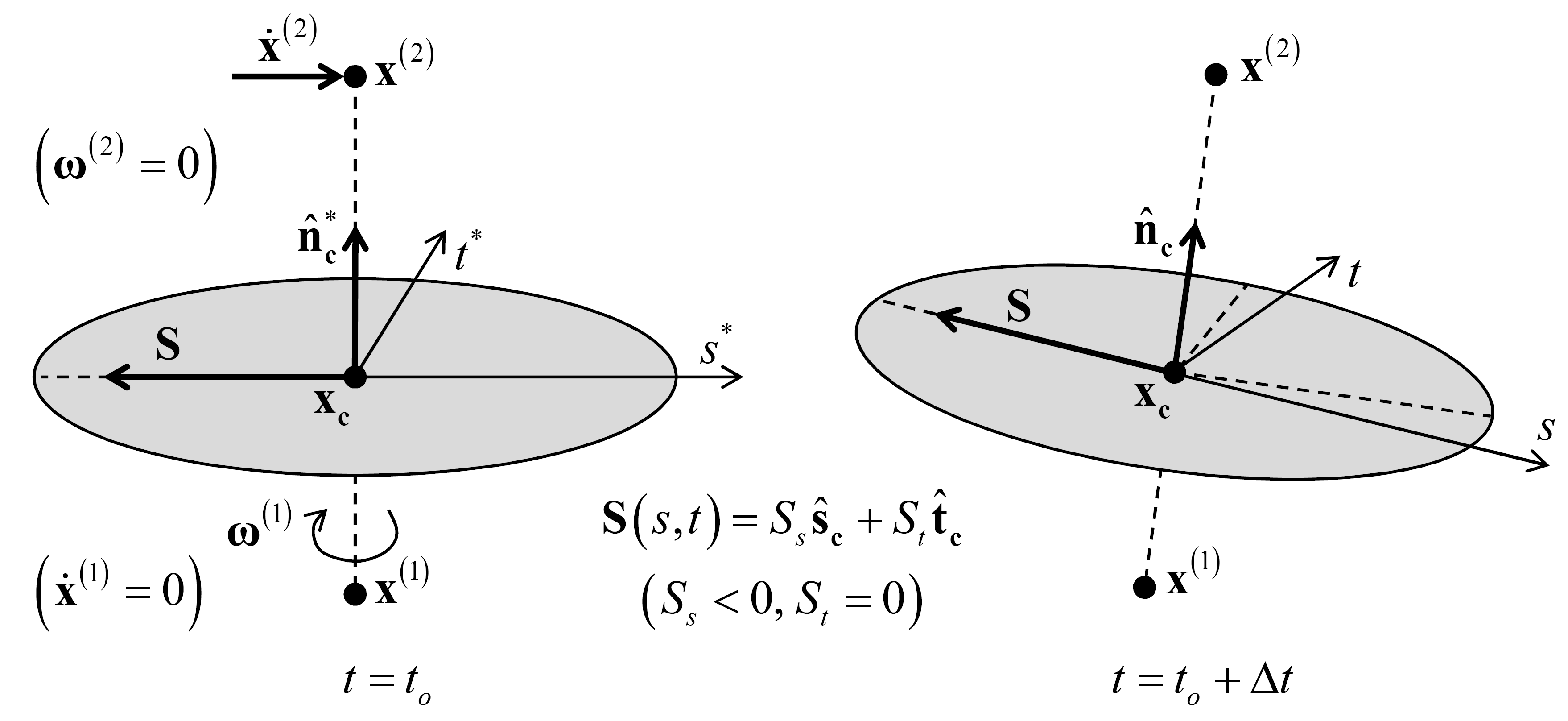
Figure 4: Orientation of contact plane and a vector that lies on the plane in response to rotation of the bottom piece and translation of the top piece.
A vector quantity that lies on the contact plane \((\mathbf{S})\) can be expressed in the contact plane coordinate system by the relations:
Relative Motion at a Contact
The relative motion of the piece surfaces at a contact is described by the relative translational \(( \dot{\pmb{δ}} )\) and rotational \(( \dot{\pmb{θ}} )\) velocities:
In this expression, \(\dot{\mathbf{x}}_\mathbf{c}^{(b)}\) is the translational velocity of body \((b)\) at the contact location:
where \(\dot{\mathbf{x}}^{\left(b\right)}\) is the translational velocity of body \((b)\); \(\pmb{ω} ^{\left(b\right)}\) is the rotational velocity of body \((b)\); \(\mathbf{x_c}\) is the contact location and \(\mathbf{x}^{\left(b\right)}\) is either the centroid (if the body is a ball or clump) or the center of rotation (if the body is a wall) of body \((b)\). See Figure 5, and note that this expression can be obtained by setting \(\mathbf{x_p} =\mathbf{x_c}\) in Equation (9). The contact location defines a point that is fixed w.r.t. each body, and thus \(\dot{\mathbf{x}}_\mathbf{c} ^{(b)}\) is the translational velocity of that point in body \((b)\).
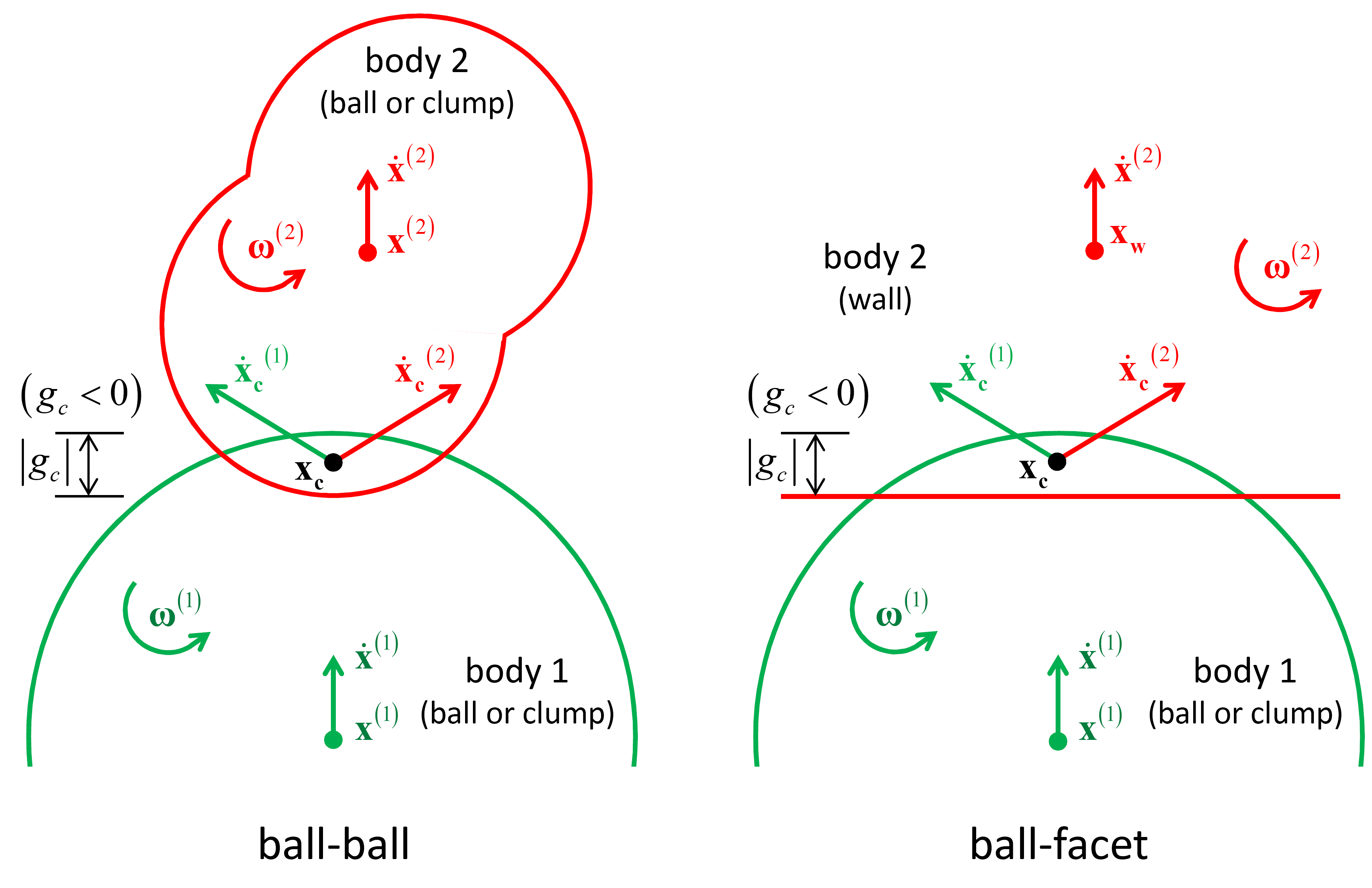
Figure 5: Body motion at a contact for the two fundamental contact types: ball-ball and ball-facet.
Each body has a reference point (\(\mathbf{x}\)) and a rotational velocity (\(\pmb{ω}\)). The reference point remains fixed w.r.t. the body. The reference point for a ball or clump is the body centroid and the reference point for a wall is the center of rotation. The translational velocity of a point \(\mathbf{x_{p}}\) that is fixed w.r.t. the body is given by
where \(\mathbf{r_{p}}\) is the relative position of the point, \(\mathbf{x}^{\left(b\right)}\) is the centroid of body (\(b\)), and \(\mathbf{x_{w}}\) is the wall center of rotation.
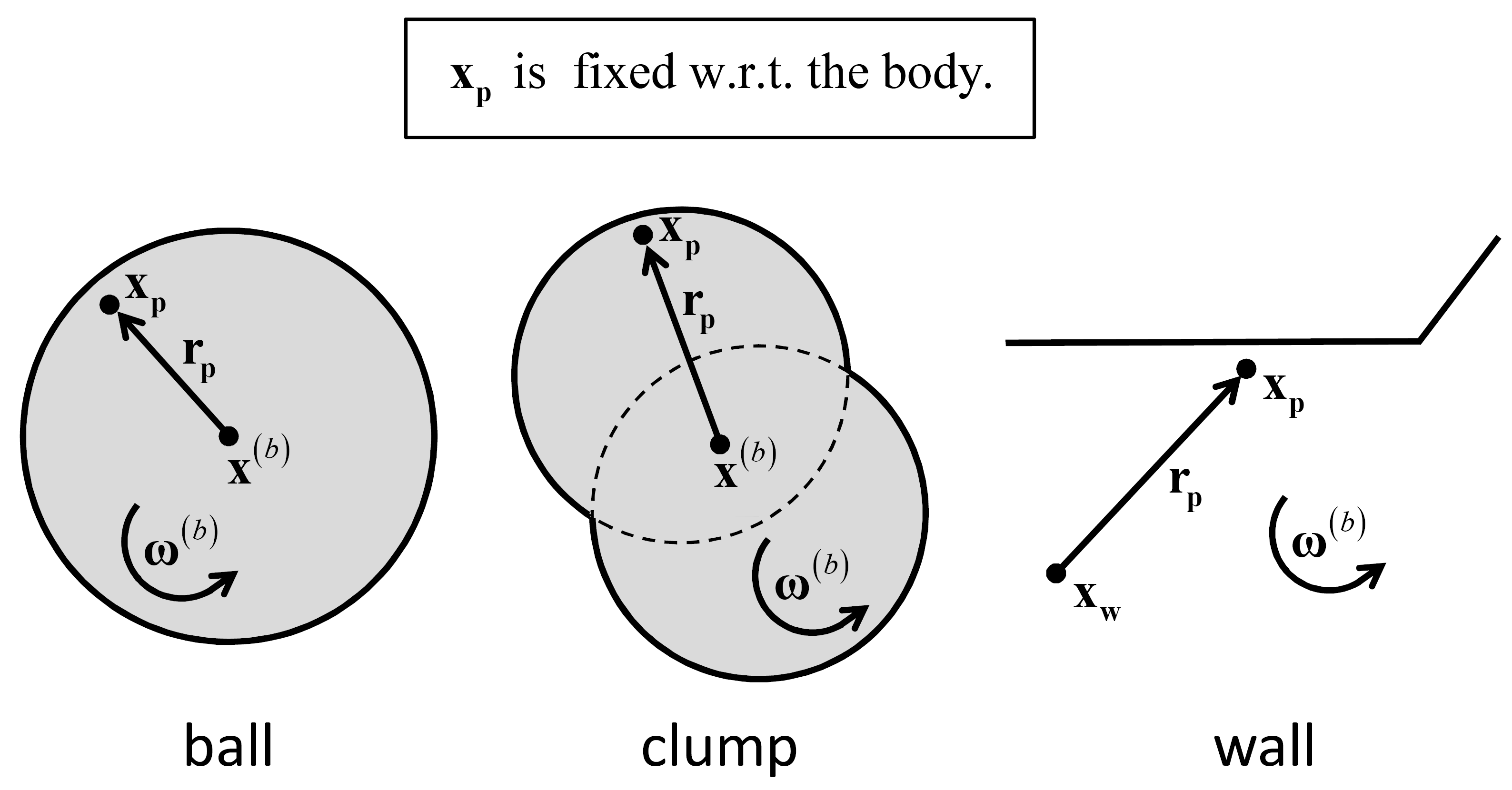
Figure 6: Kinematic variables used to describe body motion for the three fundamental body types: ball, clump, and wall.
The relative translational velocity can be expressed as
where \(\dot{\pmb{δ }}_\mathbf{n}\) (\(\dot{\delta}_{n} >0\) is moving apart) and \(\dot{\pmb{δ} }_\mathbf{s}\) are the relative translational velocities normal and tangential, respectively, to the contact plane, and the subscripts \(n\) and \(s\) correspond with normal and shear action, respectively (see Figure 7 and Figure 9—the centering of the contact within the interaction volume ensures that the relative displacement is symmetric w.r.t. the contact plane). For the 2D model, Equation (10) satisfies the condition \(\dot{\delta}_{ss} \equiv 0\).
The relative rotational velocity can be expressed as
where \(\dot{\pmb{θ} }_\mathbf{t}\) (\(\dot{\theta }_{t} >0\) is shown in Figure 8) and \(\dot{\pmb{θ} }_\mathbf{b}\) are the relative rotational velocities normal and tangential, respectively, to the contact plane, and the subscripts \(t\) and \(b\) correspond with twisting and bending action, respectively (see Figure 8 and Figure 9—the second rotation in Equation (5) ensures that the relative rotation is symmetric w.r.t. the contact plane). For the 2D model, Equation (11) satisfies the conditions: \(\dot{\pmb{θ} }_\mathbf{t} \equiv \mathbf{0}\) and \(\dot{\pmb{θ} }_\mathbf{b}\) is aligned with the \(z\) axis such that \(\dot{\theta }_{bt} \equiv 0\) and \(\dot{\theta }_{bk} =-\dot{\theta }_{bs}\).
The relative displacement and rotation increments at the contact during a timestep \(\Delta t\) are
where \(\Delta \delta _{n}\) is the relative normal-displacement increment, \(\Delta \pmb{δ} _\mathbf{s}\) is the relative shear-displacement increment, \(\Delta \theta _{t}\) is the relative twist-rotation increment, and \(\Delta \pmb{θ} _\mathbf{b}\) is the relative bend-rotation increment. For the 2D model, Equation (12) satisfies the conditions: \(\Delta \delta _{ss} \equiv \Delta \theta _{t} \equiv \Delta \theta _{bt} \equiv 0\) and \(\Delta \theta _{bk} =-\Delta \theta _{bs}\).
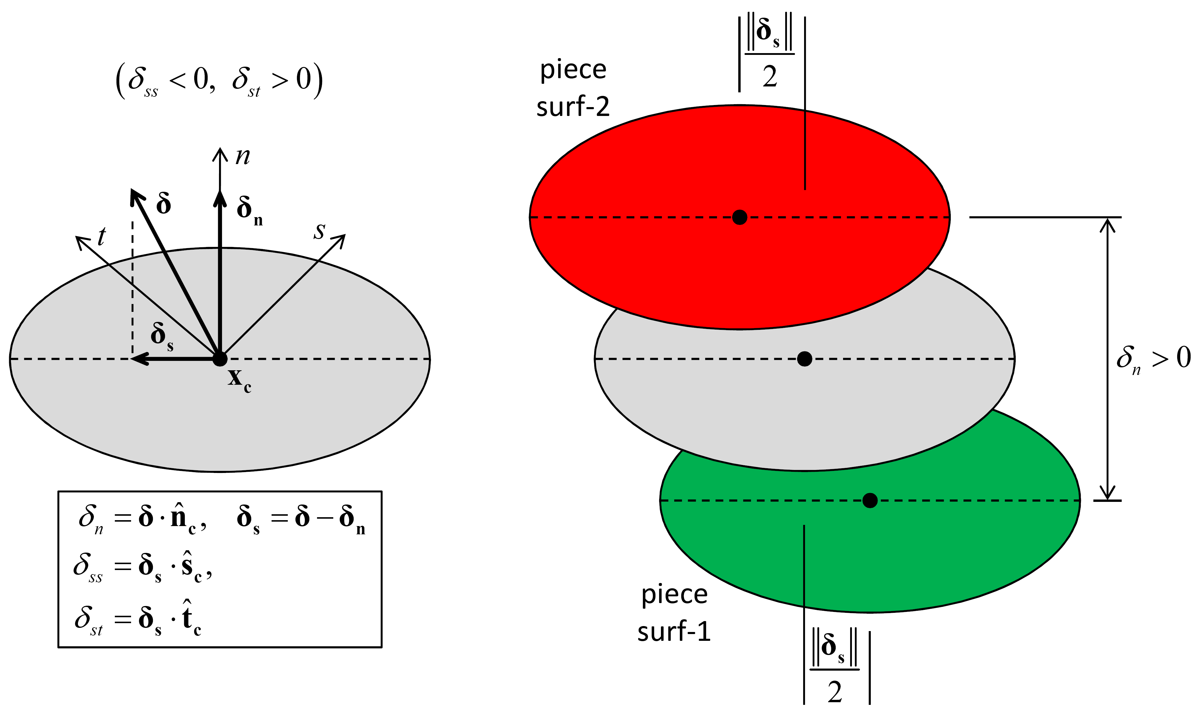
Figure 7: Kinematics of a contact showing contact plane with relative displacement and motion of piece surfaces.
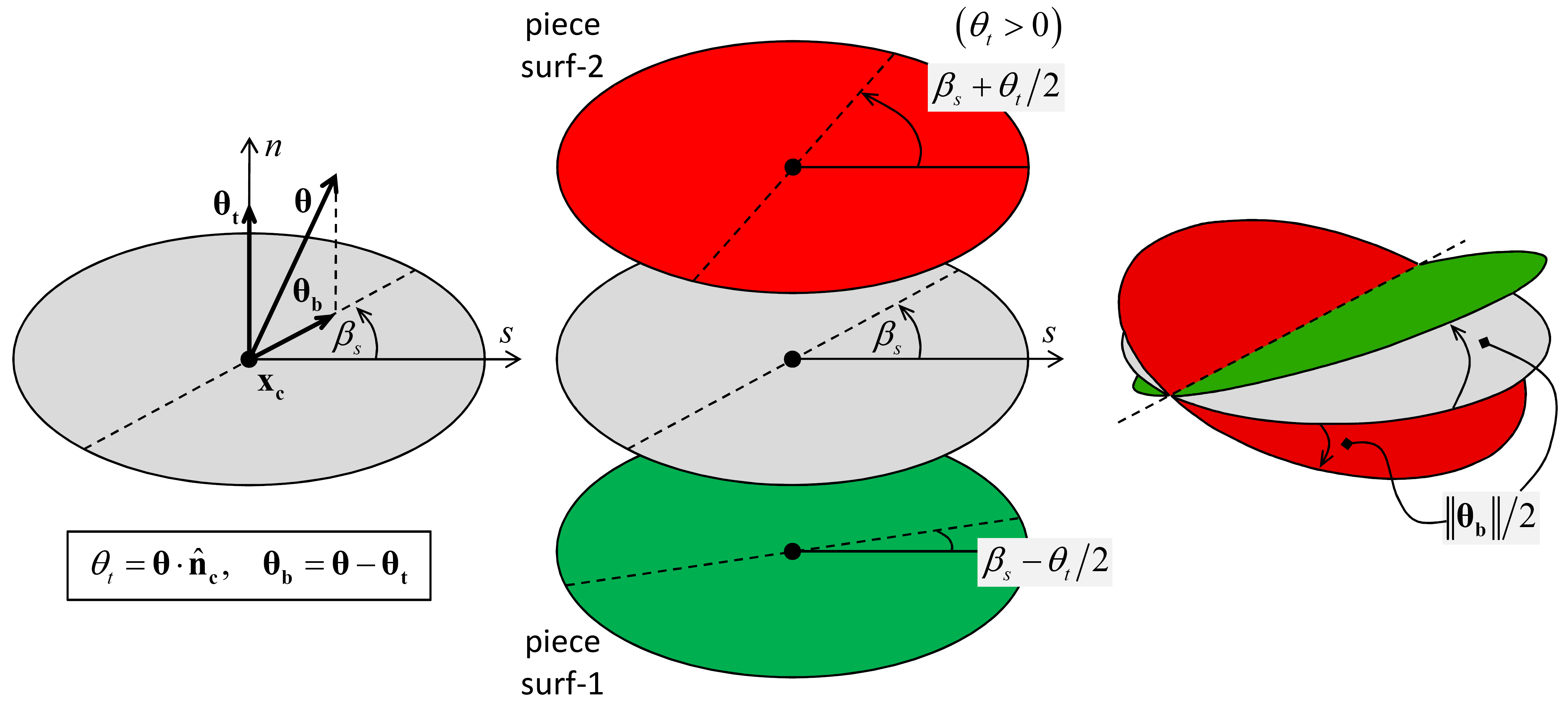
Figure 8: Kinematics of a contact showing contact plane with relative rotation and motion of piece surfaces.
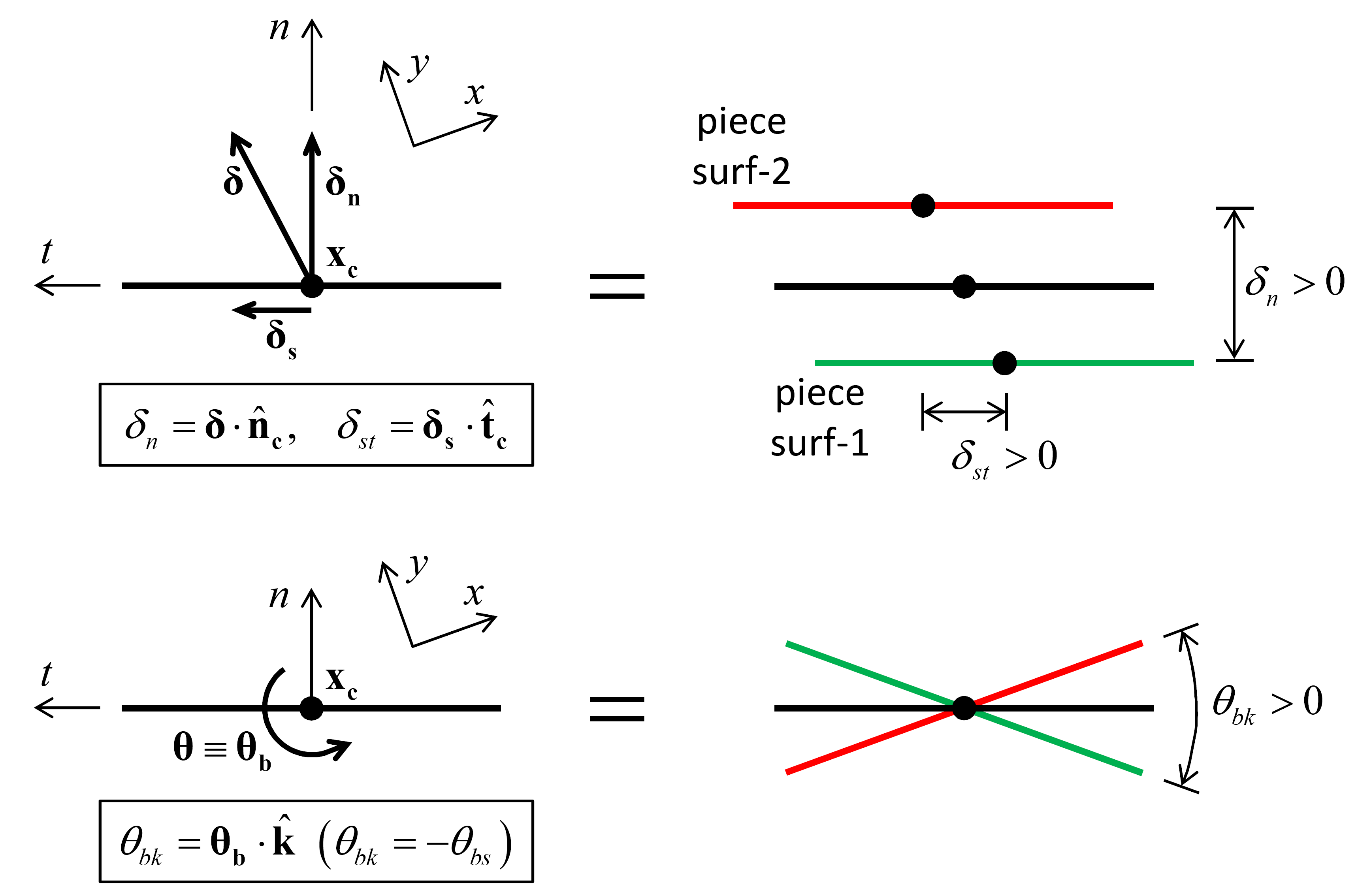
Figure 9: Kinematics of a contact for the 2D model showing contact plane with relative rotation and motion of piece surfaces.
| Was this helpful? ... | FLAC3D © 2019, Itasca | Updated: Feb 25, 2024 |