Wave Propagation in a Coupled PFC-FLAC3D model
Problem Statement
Note
To view this project in the program, use the menu command . Choose “—————/ ————–” and select “——-.—- to load. The main data file used is shown at the end of this example. The remaining data files can be found in the project.
The following example illustrates plane wave propagation through a one-dimensional “bar” using PFC-FLAC3D coupling. The bar is composed of particles bonded together on the left hand side of the system, and of zones on the right hand side. The left-hand end is a “quiet boundary” that absorbs any incident waveform. The PFC and FLAC3D regions overlap over a specified length, where they are coupled using the Ball-Zone coupling scheme. An input pulse is also injected at the left-hand boundary.
Numerical Model
The data files “wave_cpl.dat” simulate wave propagation in a bar made up of a coupled PFC-FLAC3D system. The time history of the input pulse is
where \(A\) is the amplitude of the pulse and \(f\) is the frequency. The duration of the pulse is 1\(/f\), and \(U̇\) (the velocity applied to the PFC model) is set to zero after the duration of the pulse. Parameters \(R, ρ, C, f\), and \(A\) are set in the initial section of “wave_cpl.dat”.
When the data files are executed with PFC, the time histories reproduced in Figure 1 is generated.
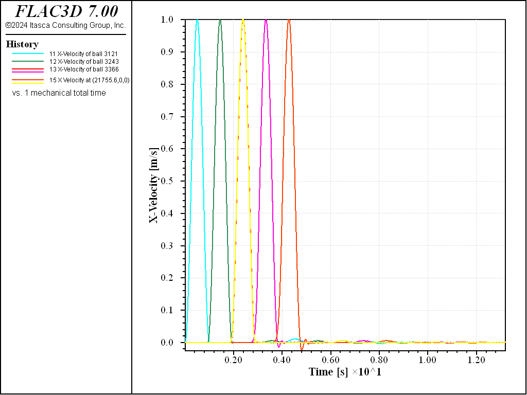
Figure 1: Velocity histories.
Data File
wave_cpl.dat
model new
model configure dynamic
model large-strain on

[wfreq  = 1.0   ] ; pulse frequency [1/s]
[wpeak  = 1.0   ] ; pulse peak velocity [m/s]
[rho    = 2700.0 ]
[emod   = 75.0e9 ]
[nu     = 0.25]
[kappa  = 15.0]
[mmod   = emod*(1-nu)/((1+nu)*(1-2.0*nu))
[cp     = math.sqrt(mmod/rho)]          ; p-wave velocity [m/s]
[cs = math.sqrt(emod/(2.0*rho*(1+nu)))] ; s-wave velocity [m/s]
[lambda = cp/(wfreq)]
[l5     = cs/(5.0)]
[rad    = 0.5*(l5/kappa)]
[rhob   = 6.0/math.pi*rho ]

[l  = 4.0*lambda]
[nb = 5]
[h  = nb*2.0*rad]
[nz = 1]
[zc = h/nz]
[cl = 10.0*zc]
[nx = int((0.5*(l+cl))/zc)]
[b_pfc = (int(0.5*l/(2.0*rad))+1)*2.0*rad-rad]
[b_f3d = b_pfc -cl]
[l     = b_f3d + nx*zc]

[epsilon = 1.0e-3]

zone create brick size [nx*nz] [nz] [nz] ...
                  point 0  [b_f3d]  [-0.5*zc] [-0.5*zc] ...
                  point 1      [l]  [-0.5*zc] [-0.5*zc] ...
                  point 2  [b_f3d]  [ 0.5*zc] [-0.5*zc] ...
                  point 3  [b_f3d]  [-0.5*zc] [ 0.5*zc]
zone cmodel assign elastic
zone property young [emod] poisson [nu]
zone initialize density [rho]
model cycle 0 ; to initialize gp masses
model range create 'right' position-x [l-0.1*zc] [l+0.1*zc]
zone face group 'right' range named-range 'right'
zone face apply quiet-normal range named-range 'right'
zone face apply quiet-dip range named-range 'right'
zone face apply quiet-strike range named-range 'right'
zone gridpoint fix velocity-y
zone gridpoint fix velocity-z

model domain extent [0.0-5.0*rad] [l+5.0*rad] ...
                    [-nb*rad-5.0*rad] [nb*rad+5.0*rad]
ball generate cubic radius [rad] box [0.0] [b_pfc] [-(nb-1)*rad] [(nb-1)*rad]
ball attribute density [rhob]
contact cmat default model linearpbond ...
                     method pb_deformability emod [4.0/math.pi*mmod] ...
                     kratio 1.0 ...
                     property pb_ten 1e20 pb_coh 1e20
model clean
contact method bond gap 0.01

ball-zone create

fish define setMassFactors(eps)
  loop foreach local cb ball.zone.ball.list
    local b = ball.zone.ball.ball(cb)
    local bxpos = ball.pos.x(b)
    ball.extra(b,1) = (1.0-2.0*eps)*(b_pfc - bxpos)/(b_pfc-b_f3d) + eps
    ball.zone.ball.mass.factor(cb) = ball.extra(b,1)
  endloop
  loop foreach local cgp ball.zone.gp.list
    local gp     = ball.zone.gp.gp(cgp)
    local gpxpos = gp.pos.x(gp)
    gp.extra(gp,1) = (1.0-2.0*eps)*(b_f3d - gpxpos)/(b_f3d - b_pfc) + eps
    ball.zone.gp.mass.factor(cgp) = gp.extra(gp,1)
  endloop
end
[setMassFactors(epsilon)]

ball group 'left' range position-x [-0.1*rad] [0.1*rad]
[mleft = ball.groupmap('left')]

history interval 1
model history name  '1' mechanical time-total
ball  history name '11' velocity-x position 0.0,0.0,0.0
ball  history name '12' velocity-x position [0.25*l],0.0,0.0
ball  history name '13' velocity-x position [0.5*l],0.0,0.0
zone  history name '14' velocity-x position [0.75*l],0,0
zone  history name '15' velocity-x position [l],0,0
zone  history name '16' velocity-x position [0.5*l],0,0
ball  history name '21' displacement-x position 0.0,0.0,0.0
ball  history name '22' displacement-x position [0.25*l],0.0,0.0
ball  history name '23' displacement-x position [0.5*l],0.0,0.0
zone  history name '24' displacement-x position [0.75*l],0,0
zone  history name '25' displacement-x position [l],0,0
zone  history name '26' displacement-x position [0.5*l],0,0

fish define pulse
  local wave = 0.0
  if mech.time.total <= 1.0 / wfreq
    wave = 0.5*(1.0 - math.cos(2.0*math.pi*wfreq*mech.time.total)) * wpeak
  endif
  loop foreach local b mleft
    ball.force.app(b,1) =  4.0*rad^2*cp*rho*wave
  endloop
end

model save 'wave-cpl_ini'
model solve time [3.5*(l/cp)] fish-call 1.0 pulse
model save 'wave-cpl_final'
program return
| Was this helpful? ... | FLAC3D © 2019, Itasca | Updated: Feb 25, 2024 |