Verification Examples
Slip on a Joint Induced by a Propagating Harmonic Shear Wave
Problem Statement
This problem concerns the effects of a planar discontinuity on the propagation of an incident shear wave. Two homogeneous, isotropic, semi-infinite elastic regions, separated by a planar discontinuity with a limited shear strength, are shown in Figure 1. A normally incident, plane-harmonic shear wave will cause slip at the discontinuity, resulting in frictional energy dissipation. Thus, the energy will be reflected, transmitted and absorbed at the discontinuity. The problem is modeled with 3DEC, and the results are used to determine the coefficients of transmission, reflection and absorption. These coefficients are compared with ones given by an analytical solution (Miller 1978).
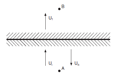
Figure 1: Transmission and reflection of incident harmonic wave at a discontinuity.
Analytic Solution
The coefficients of reflection (R), transmission (T ) and absorption (A) given by Miller (1978) for the case of uniform material are
where \(E_I\), \(E_T\) and \(E_R\) represent the energy flux per unit area per cycle of oscillation associated with the incident, transmitted and reflected waves, respectively. The coefficient \(A\) is a measure of the energy absorbed at the discontinuity. The energy flux \(E_I\) is given by
where:
\(T\) = \((2 \pi) / \omega\) = the period for the incident wave;
\(\sigma_s\) = shear stress;
\(v_s\) = particle velocity in the \(x\)-direction; and
\(\omega\) = frequency of incident wave (radian/sec).
For elastic media,
Hence,
in which \(c\) is the velocity of the propagating shear wave.
The energy flux of the incident wave, \(E_I\), is evaluated at Point A (see Figure 1) for no slip at the discontinuity. The energy flux of the transmitted wave, \(E_T\), is evaluated at Point B for the case of slip at the discontinuity. The energy flux of the reflected wave, \(E_R\), is calculated by determining the difference of velocities in two cases: slip and no slip.
Numerical Model
The numerical results are determined for four values of the dimensionless frequency \(\omega \gamma U/\tau_s\), where \(\gamma = (\rho G)^{1/2}\), \(\tau_s\) = discontinuity cohesion, \(U\) = displacement amplitude of incident wave, \(\rho\) = density of the media, and \(G\) = shear modulus of the media.
The problem geometry modeled by 3DEC is shown in Figure 2. The media were modeled with elastic, fully deformable blocks of height (\(h/ 2\)), width \(b\) and length \(l\). The blocks are separated by a planar discontinuity extending in the \(xz\)-plane. The blocks were internally discretized into tetrahedral zones, as shown in Figure 3. Nonreflecting boundary conditions were used on the top and bottom of the model. Displacements at boundaries along the \(yz\)-plane at \(x\) = 0 and \(x\) = \(b\) were restrained in the \(y\)-direction to simulate plane shear wave conditions. Displacements at boundaries were restrained in the \(z\)-direction along the \(xy\)-plane at \(z\) = 0 and \(z\) = l to simulate the plane-strain condition.
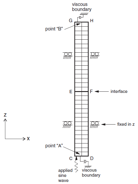
Figure 2: Geometry for the problem of slip induced by harmonic shear.
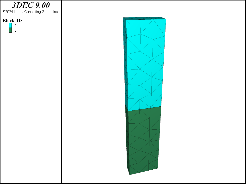
Figure 3: 3DEC block model showing internal discretization.
Material Properties
The material properties of the elastic media and planar discontinuity are given in the following two tables.:
Mass density |
2,650 kg/m3 |
Shear modulus |
10,000 MPa |
Bulk modulus |
16,667 MPa |
Normal stiffness |
10,000 MPa/m |
Shear stiffness |
10,000 MPa/m |
Friction angle |
0 |
Cohesion |
2.5, 0.5, 0.1 and 0.02 MPa |
Dynamic Loading
The harmonic shear stress applied at the bottom boundary has the following characteristics:
maximum stress of incident wave: 1.0 MPa
frequency of incident wave: 1 Hz
type of harmonic wave: sinusoidal
Note that the magnitude of the incident wave must be doubled in the numerical model to account for the simultaneous presence of the nonreflecting boundary.
Results
The analytical solution for wave propagation through a slipping discontinuity (Miller 1978) assumes a Mohr-Coulomb discontinuity failure criterion with constant cohesion. In 3DEC, this is accomplished by setting the residual cohesion (cohesion-residual) equal to the cohesion. By default, the cohesion drops to 0 when slip occurs. The same thing is done for tension.
An initial run assumed that the discontinuity remains elastic by setting the discontinuity cohesion to 2.5 MPa. A stress wave of amplitude 1 MPa and frequency 1 Hz was applied at the base of the model. It should be noted that the displacements and velocities are determined at the nodal points of the tetrahedron. The stresses, however, are determined at the centroid of the tetrahedron. The time histories of shear stress, velocity and displacement are monitored at Points A (40, 15, −200) and B (40, 15, 200). The linear history of stresses are monitored close to Points A and B. The shear stresses at Points A and B are shown in Figure 4. From the amplitude of the stress history at A and B, it is clear that there was perfect transmission of the wave through the discontinuity. It is also clear from Figure 4 that the nonreflecting boundary condition provides perfect absorption of normally incident waves.
In the next run, the cohesion was lowered to 0.5 MPa to permit slip along the discontinuity. The recorded shear stresses at Points A and B are shown in Figure 5. The peak stress at Point A is the superposition of the incident wave and the wave reflected from the slipping discontinuity. Figure 6 and Figure 7 show the shear stress at Points A and B for a discontinuity cohesion of 0.1 and 0.02 MPa. It can be seen in Figure 5 through Figure 7 that the shear stress of Point B is limited by the discontinuity strength at 0.5, 0.1, and 0.02 MPa, respectively.
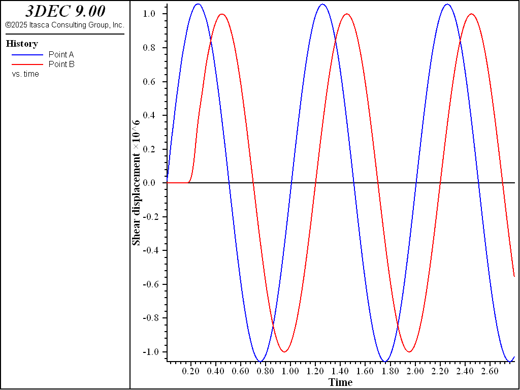
Figure 4: Shear stress vs time at Points A and B for the case of an elastic discontinuity (cohesion = 2.5 MPa).
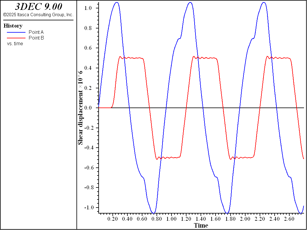
Figure 5: Shear stress vs time at Points A and B for the case of an elastic discontinuity (cohesion = 0.5 MPa).
Figure 6: Shear stress vs time at Points A and B for the case of an elastic discontinuity (cohesion = 0.1 MPa).
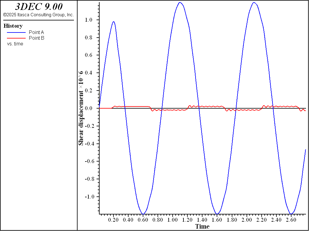
Figure 7: Shear stress vs time at Points A and B for the case of an elastic discontinuity (cohesion = 0.02 MPa).
The energy flux, \(E_I\), is evaluated using Equation (2) at Point A for non-slipping discontinuities (i.e., cohesion = 2.5 MPa). \(E_T\) is evaluated at Point B for the slipping discontinuity (i.e., cohesion = 0.5, 0.1 and 0.02MPa). \(E_R\) is determined at PointB by taking the difference in velocity from the runs with slipping and non-slipping discontinuities. The coefficients of reflection (R), transmission (T ), and absorption (A) are computed using Equation (1) (see FISH function energy in file “sihsw.fis” below), and are plotted in Figure 8, along with the analytical solution (Miller 1978). The 3DEC results agree very well with the analytical solution (Figure 8).
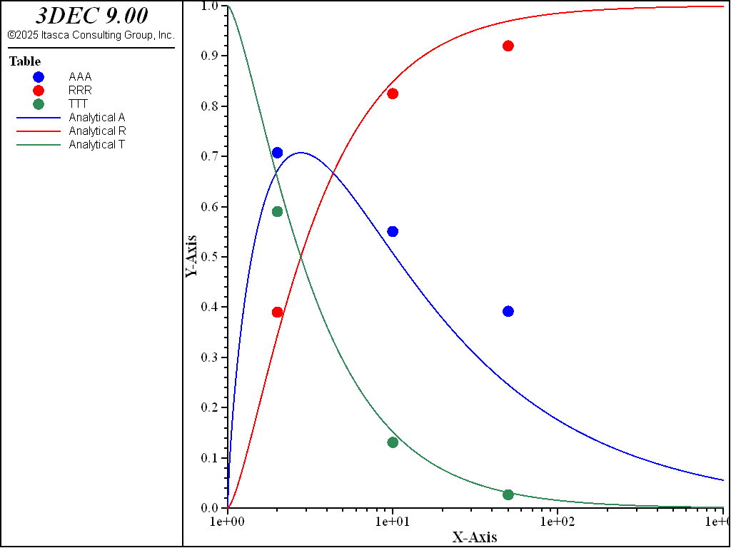
Figure 8: Comparison of transmission, reflection, and absorption coefficients.
Data File
;---------------------------------------------------------------------
; script file forigin dynamic problem 'Slip induced by harmonic wave'
;---------------------------------------------------------------------
model new
fish automatic-create off

model title "Slip induced by harmonic wave"

model configure dynamic
model large-strain on

fish define setup
    global mat_shear = 1e10
    global mat_dens  = 2650
    global freq       = 1.0
    global tload     = 10.0
    global w         = 2.0 * math.pi * freq
    global height = 400.0
end
[setup]

block create brick 0,80 0,30 -200,200
block cut joint-set dip-direction=90 dip 0 origin 80,0,0
;
block zone generate edgelength 31
;
block zone cmodel assign elastic
block zone property density=[mat_dens] bulk=16.667e9 shear=[mat_shear]
;
; set viscous boundary along xy plane at z=-200 and z=200
block gridpoint apply viscous-x viscous-z range position-z -200
block gridpoint apply viscous-x viscous-z range position-z 200
;
; set roller boundary along xz plane at y=0 and y=30
block gridpoint apply velocity-y=0 range position-y 0
block gridpoint apply velocity-y=0 range position-y 30
;
;  set zvel=0 along yz plane at x=0 and x=80
block gridpoint apply velocity-z=0 range position-x 0
block gridpoint apply velocity-z=0 range position-x 80
;
; shear stress along xz plane at z=-200
; set sinusoidal wave function forigin the
; applied stress at the boundary
; freq = 1 Hz[freq = 10.0]

fish define sin_
  sin_ = math.sin(2.0*math.pi*mech.time*freq)
end


block face apply stress-xz 2e6 fish sin_  range position-z -200

; set histories
history interval=10
block history name 'Point A' stress-xz  position 40,15,-200
block history name 'Point B' stress-xz  position 40,15,200
block history name 'v1' velocity-x position (40,15,-200)
block history name 'v2' velocity-x position (40,15,200)
block history name 'd1' displacement-x position (40,15,-200)
block history name 'd2' displacement-x position (40,15,200)
model history name 'time' dynamic time-total

program call "sihsw.fis"
model save 'dint_ini'

; joint is elastic
block contact jmodel assign elastic
block contact property stiffness-normal=10.0e9 stiffness-shear=10.0e9
block contact material-table default property stiffness-normal=10.0e9 ...
                                          stiffness-shear=10.0e9

model cycle 3000
history export 'v1' vs 'time' table '1'
table '1' export 'elastic' truncate
[find_u]
model save "dinte"

; ---cohesion 0.5 ---
model restore "dint_ini"

; joint is perfectly plastic
block contact jmodel assign mohr
block contact property stiffness-normal=10.0e9 stiffness-shear=10.0e9 ...
    cohesion=0.5e6 cohesion-residual 0.5e6 ...
    tension=1e12 tension-residual 1e12
block contact material-table default property stiffness-normal=10.0e9 ...
                                          stiffness-shear=10.0e9
model cycle 3000

table '1' import 'elastic'
history export 'v1' vs 'time' table '2'
history export 'v2' vs 'time' table '3'
[energy(0.5e6)]

; create and export tables forigin comparison with analytical solution
table '10' export 'AAA' truncate
table '11' export 'RRR' truncate
table '12' export 'TTT' truncate
model save "dint0p5"

; --- cohesion 0.1 ---
model restore "dint_ini"

block contact jmodel assign mohr
block contact property stiffness-normal=10.0e9 stiffness-shear=10.0e9 ...
    cohesion=0.1e6 tension=1e12 cohesion-residual 0.1e6 tension-residual 1e12
block contact material-table default property stiffness-normal=10.0e9 ...
                                          stiffness-shear=10.0e9

model cycle 3000
table '1' import 'elastic'
history export 'v1' vs 'time' table '2'
history export 'v2' vs 'time' table '3'
; import existing tables origin results so new values are appended
table '10' import 'AAA'
table '11' import 'RRR'
table '12' import 'TTT'
[energy(0.1e6)]

; now export
table '10' export 'AAA' truncate
table '11' export 'RRR' truncate
table '12' export 'TTT' truncate
model save "dint0p1"

; --- cohesion 0.1 ---
model restore "dint_ini"

block contact jmodel assign mohr
block contact property stiffness-normal=10.0e9 stiffness-shear=10.0e9 ...
   cohesion=0.02e6 tension=1e12 cohesion-residual 0.02e6 tension-residual 1e12
block contact material-table default property stiffness-normal=10.0e9 ...
                                          stiffness-shear=10.0e9

model cycle 3000
table '1' import 'elastic'
history export 'v1' vs 'time' table '2'
history export 'v2' vs 'time' table '3'
table '10' import 'AAA'
table '11' import 'RRR'
table '12' import 'TTT'
[energy(0.02e6)]
table '10' export 'AAA' truncate
table '11' export 'RRR' truncate
table '12' export 'TTT' truncate
model save "dint0p02"

; --- get analytical solution ---
model new
table '10' import 'AAA'
table '11' import 'RRR'
table '12' import 'TTT'
table '10' label 'AAA'
table '11' label 'RRR'
table '12' label 'TTT'
program call "sihsw-ana.fis"
[analytical_table]
model save 'anal_tables'
Fish File
;--------------------------------------------------------------------------
; FISH functions for dynamic problem 'Slip induced by harmonic wave'
;---------------------------------------------------------------------------

fish define ini_time
  global speed = math.sqrt(mat_shear/mat_dens)
  global time0 = 0.0
  global time1 = height/speed
  global time2 = time1 + 1./freq
end
[ini_time]

fish define find_u
    command
        history export 'd1' vs 'time' table '4'
    end_command
    local pnt = table.get(4)
    local s = table.size(pnt)
    local max_disp = 0.0
    local min_disp = 1e20
    loop local i (1,s)
        local time = table.x(pnt,i)
        if time >= time1 then
            if time <= time2 then
                local val = math.abs(table.y(pnt,i))
                max_disp = math.max(max_disp,val)
                min_disp = math.min(min_disp,val)
            end_if
        end_if
    end_loop
    global UUU = (max_disp - min_disp) * 0.5

    ; write to file for use later
    local status = file.open('ufile.txt',1,1)
    local line = array.create(1)
    line(1) = UUU
    status = file.write(line,1)
    status = file.close
end

fish define read_u
  local status = file.open('ufile.txt',0,1)
  local line = array.create(1)
  file.read(line,1)
  UUU = float(line(1))
end

fish define energy(cohesion) ;- compute energy coefficients
                             ;  for slipping-joint example  -
    ; table 1 - x-velocity at point A for elastic joint case
    ; table 2 - x-velocity at point A for slipping joint case
    ; table 3 - x-velocity at point B for slipping joint case
    ; table 10 - A values for all cases
    ; table 11 - R values for all cases
    ; table 12 - T values for all cases
    ; Ei - energy flux for incident wave
    ; Et - energy flux for transmitted wave
    ; Er - energy flux for reflected wave
    ; AAA  - a measure of energy absorbed at the interface
    ; Places AAA, RRR, TTT results in A, R, T tables
    local Cs     = math.sqrt(mat_shear / mat_dens)
    local factor = mat_dens * Cs
    local Ei    = 0.0
    local Et    = 0.0
    local Er    = 0.0
    local t_n_1 = 0.0
    local AAA   = 0.0
    local TTT   = 0.0
    local RRR   = 0.0
    local items = table.size(1)
    loop local i (1,items)
        local t_n = table.x(1,i)
        local d_t  = t_n - t_n_1
        t_n_1 = t_n
        local Vsa_e = table.y(1,i)
        local Vsa_s = table.y(2,i)
        local Vsb_s = table.y(3,i)
        Ei = Ei + factor * Vsa_e * Vsa_e * d_t
        Et = Et + factor * Vsb_s * Vsb_s * d_t
        Er = Er + factor * (Vsa_s-Vsa_e) * (Vsa_s-Vsa_e) * d_t
    end_loop
    RRR = math.sqrt(Er/Ei)
    TTT = math.sqrt(Et/Ei)
    AAA = AAA + math.sqrt(1.0-RRR*RRR-TTT*TTT)

    ; for analytical solution
    read_u
    local g = math.sqrt(mat_dens*mat_shear)
    local x = (w * g * UUU) / cohesion

    local aaatab = table.get(10)
    table(aaatab,x) = AAA

    local rrrtab = table.get(11)
    table(rrrtab,x) = RRR

    local ttttab = table.get(12)
    table(ttttab,x) = TTT
end
Line Source in an Infinite Elastic Medium with a Discontinuity
Problem Statement
This problem concerns the dynamic behavior of a single discontinuity under explosive loading. The problem, shown in Figure 9, consists of a planar crack of infinite lateral extent in an elastic medium, and a dynamic load at some distance, \(h\), from the discontinuity. This problem was modeled using 3DEC to determine the dynamic response of the discontinuity for a line source (in the \(z\)-direction). The slip of the interface at a Point P, obtained by numerical analysis using 3DEC, is compared with the closed-form solution derived by Day (1985).
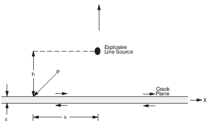
Figure 9: Problem geometry for an explosive source near a slip-prone discontinuity.
Analytic Solution
The closed-form solution for crack slip as a function of time was derived by Day (1985) and is given by
where
\(r\) = \((x^2 + h^2)^{1/2}\), distance from the point source to the point on the crack where the slip is monitored;
\(H(\tau)\) = step function;
\(\tau\) = \(t - (r/\alpha)\);
\(m_o\) = source strength;
\(\alpha\) = velocity of pressure wave;
\(\beta\) = velocity of shear wave;
\(\rho\) = density;
\(\eta_\alpha\) = \({(\alpha^{-2} - p^2)}^{1/2}, Re\ \eta_\alpha\ \ge\ 0\);
\(\eta_\beta\) = \({(\beta^{-2} - p^2)}^{1/2}, Re\ \eta_\beta \ \ge\ 0\);
\(R(p)\) = \({(1 - 2\beta^2\ p^2)}^2 + 4\beta^4\ \eta_\alpha\ \eta_\beta\ p^2 + 2\beta\ \eta_\beta\ \gamma\); and
\(p~\) = \({{1} \over {r^2}} \biggl[ \ \bigl(\tau + {{r} \over {\alpha}}\bigr)x + i\bigl(\tau + {{2r} \over {\alpha}}\bigr)^{1/2}\ \tau^{1/2}\ h\ \biggr]\).
The slip response of the discontinuity for any source history, \(S(t)\), can be obtained by convolution of Figure 9 and the source function, \(S(t)\):
Figure 10 shows the dimensionless analytical results of slip history at a Point P for a smooth step function, and for the following values of the variables: \(\alpha^2 = 3\beta^2\), \(h = x\) and \(\gamma = 0\). The analytic solution is implemented in FISH function ana slp (listed below).
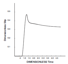
Figure 10: Dimensionless analytical results of slip history at Point P (dimensionless slip = \((4h \rho \beta^2/m_o)\delta u\), dimensionless time = \(t\beta / h\)) (Day 1985).
Model Setup
Figure 11 shows the problem geometry modeled by 3DEC. The source is located at A (\(x\) = 0 and \(z\) = 2 \(h\)), and the discontinuity is located at \(z = h\). The dynamic input was applied at the semicircular boundary of radius 0.05 h. The slip movement was monitored at Point P on the discontinuity.
The continuous medium was modeled with elastic, fully deformable blocks, as shown in Figure 12, and each block was further discretized into tetrahedral zones. In order to generate only one zone in the \(y\)-direction, the thickness of the block in the \(y\)-direction and the average edge length of the tetrahedron were assumed to be the same. The average edge length was 0.065 \(h\). All of the joints except the discontinuity were “joined” in order to model a continuous elastic medium. The discontinuity was assigned a high normal stiffness and high tensile strength in order to meet the assumption implied in the analytical solution.
Nonreflecting boundary conditions were applied along the horizontal boundaries at the top and bottom of the model and along the vertical boundary at \(x\) = 4 \(h\). A symmetric boundary condition was applied along the vertical boundary at \(x\) = 0. In order to simulate plane-strain conditions, displacement in the \(y\)-direction is restrained along \(xz\)-planes at \(y\) = 0 and \(y\) = 0.065 \(h\).
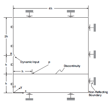
Figure 11: Problem geometry and boundary conditions for numerical model.
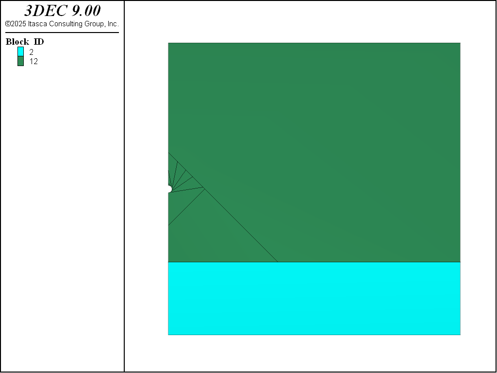
Figure 12: 3DEC model showing semicircular source and “joined” blocks used to provide appropriate zoned discretization.
Properties of Joints and Continuous Medium
The following properties were used for the elastic blocks.
Geometric scale |
\(h\) = 10, 000 MPa/m |
Mass density |
10,000 MPa/m |
Shear modulus |
100 Pa |
Bulk modulus |
166.67 Pa |
The Mohr-Coulomb joint constitutive relation was used in the analysis. The specific 3DEC parameters used for the joint relation are listed below.
Normal stiffness |
10,000 Pa/m |
Shear stiffness |
0.1 Pa/m |
Friction angle |
0 |
Cohesion |
0 |
Dynamic Loading
Radial velocities corresponding to the dynamic solution for a line source in an infinite medium were enforced at the semicircular boundary. To avoid problems with the singularity at the source, dynamic input was applied over a surface 0.05 \(h\) from the nominal point source.
3DEC analysis with both velocity and pressure input showed that velocity input gives a better match with the analytical solution than pressure input. The velocity boundary provides a more accurate representation of the dynamic stress than the pressure boundary, because in pressure input, the source function is simply scaled by static stress magnitude and neglects the inertial effects of dynamic stress at the input boundary.
The radial displacement for a line source given by Lemos (1987) is
where \(r\) is the radial distance.
The corresponding velocity is
The actual input velocity record at \(r = 0.05 h\), as shown in Figure 13, was obtained by convoluting Equation (4) and Equation (3).
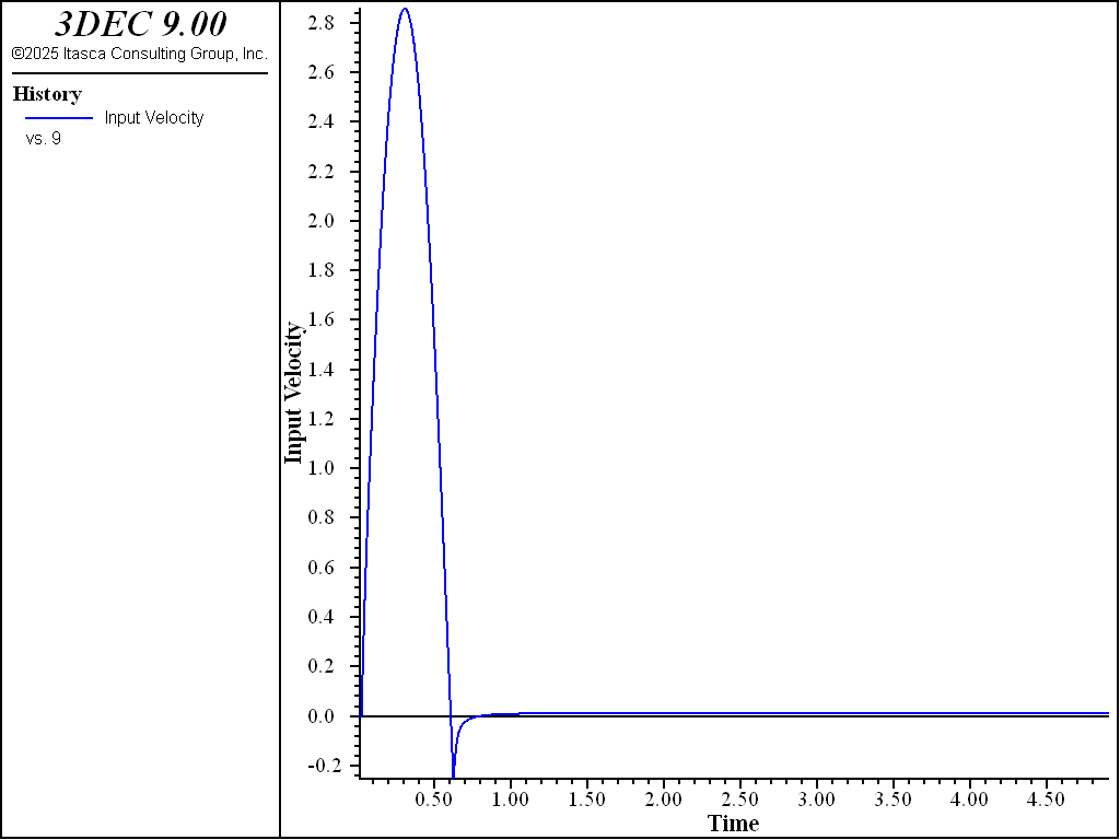
Figure 13: Input radial velocity time history prescribed at \(r = 0.05\ h\) (dimensionless velocity = \((h^2\rho\beta / m_o)v\), dimensionless time = \(\tau\beta/ h)\).
Velocity history at the boundary at \(r = 0.05 h\) is calculated in the FISH function vel inp (listed below).
Results
The dimensionless slip at Point P is plotted against the dimensionless time, and is shown in Figure 14. The dimensionless slip is compared with the analytical solution given by Day (1985). Velocity input was used on the semicircular region at \(r = 0.05 h\) for 3DEC. The error at the peak slip for 3DEC is 1.7%.
The results shown in Figure 14 were obtained with a mesh of maximum zone length of 0.065 \(h\). The slip response on the discontinuity involves higher frequency components because of zero friction along the discontinuity. This requires a finer mesh for accurate representation.
The dimensionless slip in Figure 14 for 3DEC analysis shows a good agreement with the analytical solution until the dimensionless time of 1.49. The results show, after dimensionless time of 1.49, a considerable deviation, which can be attributed to boundary reflections.
Nonreflecting boundaries are used along the top, bottom, and right-hand side boundaries. Such viscous boundaries, designed to absorb normally incident \(p-\) and \(s\)-waves, cannot be fully effective in this dynamic slip problem because the discontinuity crosses the boundary. Viscous boundaries, however, are preferable to roller boundaries.
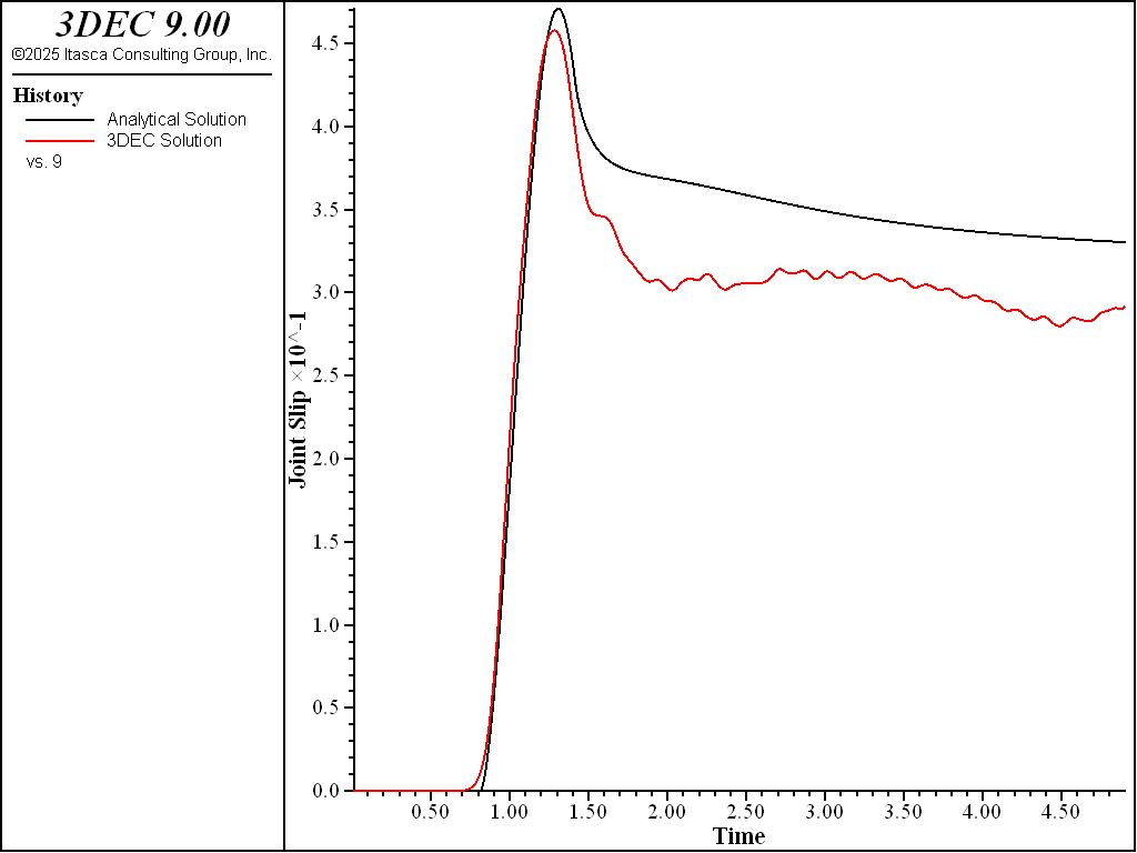
Figure 14: Comparison of dimensionless slip at Point P with Coulomb joint model (dimensionless slip = \((4h\rho\beta^2/ m_o)\delta u\), dimensionless time = \(\tau\beta/h\)).
Data File - Line Source
;==========================================================================
; verification test -- 3dec modeling of slipping crack under dynamic load
; Joint Model: Mohr-Coulomb Model
; elastic blocks
;
; dynamic analysis
;==========================================================================
;
model new
model random 10000
model configure dynamic
model large-strain on

; --- geometry ---
block create brick 0,40 0,0.65 0,40
;
block cut joint-set dip 0 dip-direction 0 origin 0,0,10
block hide range position-x 0,40 position-y 0,10 position-z 0,10
block cut joint-set dip 45 dip-direction 90 origin 0,0,25 join
block hide range plane dip 45 dip-direction 90 origin 0,0,25 above
block cut joint-set dip 45 dip-direction 270 origin 0,0,15 join
;
block hide off
block cut tunnel ...
   face-1 0,0,20.5 0.19,0,20.46 .35,0,20.35 0.46,0,20.2 .5,0,20.0 ...
              .46,0,19.8 0.35,0,19.64 .19,0,19.53 0.0,0,19.5 ...
   face-2 0,.65,20.5 0.19,.65,20.46 .35,.65,20.35 0.46,.65,20.2 ...
       .5,.65,20.0 .46,.65,19.8 0.35,.65,19.64 .19,.65,19.53 0.0,.65,19.5 ...
   group 'tunnel'
;
block delete range group 'tunnel'
block zone generate edgelength 0.650
model save "day3d-zoned"

model restore "day3d-zoned"

; --- properties ---
block zone cmodel assign elastic
block zone property density=1.0 bulk=166.67 shear=100.0
block contact jmodel assign mohr
block contact property stiffness-normal 1e4 stiffness-shear 0.1 tension 1e6
block contact material-table default property stiffness-normal 1e4 ...
                                          stiffness-shear 0.1
;
; --- boundary conditions
block gridpoint apply viscous-x viscous-z range position-z 0 ; xz plane at z=0
block gridpoint apply viscous-x viscous-z range position-z 40  ; xz plane at z=40
block gridpoint apply viscous-x viscous-z range position-x 40  ; xz plane at x=40
;
; set roller boundary along xz plane at y=0 and y=0.65
block gridpoint apply velocity-y=0 range position-y 0.0
block gridpoint apply velocity-y=0 range position-y 0.65
;  set symm boundary at x=0
block gridpoint apply velocity-x=0 range position-x -1 .5

; set velocity boundary condition along cylindrical notch
program call "vel_inp.fis"
program call "ana_slp.fis"
model cycle 1
program call "day3d.fis"
[_load( 0.0, 20.0, 0.5)]
;
block insitu  stress -1.0e-9 -1.0e-9 -1.0e-9 0 0 0

; set histories
history interval=10
fish history dtime_
fish history name 'Input Velocity' bvel_
fish history name 'Analytical Solution' aslip_
fish history name '3DEC Solution' nslip1_
fish history nslip2_
block history velocity-x position 0.5 20 0.3
block history velocity-z position 0 20.5 .03
block history velocity-z position 0 19.5 0.03
model history dynamic time-total

fish callback add _compare 1
model cycle 4000
model save "day3d"
Fish File
;=====================================================
;
; calculates unit forces on the contour of the opening
;
;=====================================================
;
fish define _load(xc_, zc_, dist_)
  loop foreach igp_ block.gp.list
      x_ = block.gp.pos.x(igp_)
      z_ = block.gp.pos.z(igp_)
      d_ = math.sqrt((x_-xc_)*(x_-xc_)+(z_-zc_)*(z_-zc_))
      if math.abs(d_-dist_) < 0.05*dist_
        nx_ = (x_-xc_)/d_
        nz_ = (z_-zc_)/d_
        gp_id = block.gp.id(igp_)
        command
          block gridpoint apply velocity-x [nx_] velocity-z [nz_] ...
                          table [_vtab] range id [gp_id]
        end_command
      end_if
  end_loop
end

;=====================================================
;
; finds contacts closest to the point of interest
; input 2 vectors
;
;=====================================================
fish define _find(f_, b_)
  global v_s_
  global h_n_
  global rho_
  global m0_
  dfmax_ = 1.e30
  dbmax_ = 1.e30
  loop foreach icx_ block.subcontact.list
      pos_ = block.subcontact.pos(icx_)
      df_= math.mag(pos_ - f_)
      db_= math.mag(pos_ - b_)
      if df_ < dfmax_ then
        dfmax_ = df_
        icf_   = icx_
      end_if
      if db_ < dbmax_ then
        dbmax_ = db_
        icb_   = icx_
      end_if
  end_loop
  vscale_ = m0_/(h_n_*h_n_*rho_*v_s_)
  dscale_ = 0.25*m0_/(h_n_*rho_*v_s_*v_s_)
end

[v_s_=10.]
[h_n_=10.]
[rho_=1.]
[m0_=1.]
[_find( (10,10,0), (10,10,0.65) )]

;=====================================================
;
; stores analytical solution in the histories, and
; convertes numerical solution in the dimensionless
; form
;
;=====================================================
[nslip1_max = 0.0]
[aslip_max = 0.0]
fish define _compare
  ;while_stepping
  dtime_ = dynamic.time.total*v_s_/h_n_
  bvel_  = table(_vtab,dynamic.time.total)/vscale_
  aslip_ = table(_utab,dtime_)
  slip1_ = block.subcontact.disp.shear(icf_)
  slip2_ = block.subcontact.disp.shear(icb_)
  nslip1_ = math.mag(slip1_)/dscale_
  nslip2_ = math.mag(slip2_)/dscale_
  nslip1_max = math.max(nslip1_max,nslip1_)
  aslip_max = math.max(aslip_max,aslip_)
end
Fish File - Velocity Input
;=====================================================
;
;  Fish function for generating the radial velocity
;  input profile at r=0.05h
;
;  Input:
;         vl   --- P-wave velocity
;         per  --- period of wave
;         tt   --- total time
;         xd   --- horizontal distance
;         nt   --- total number of dat points
;
;  Output:
;         velocity profile stored in table 1
;=====================================================
;
fish define ini_par
    vl = 0.0
    per = 0.0
    tt = 0.0
    xd = 0.0
    nt = 1000
    _vtab  = '1' ; table storing velocity profile
    _fptab = '2'
    _vhtab = '3'
end
[ini_par]
;
fish define vel_inp
   if xd <= 0.0
      exit
   endif
   if per <= 0.0
      exit
   endif
   _w  = 2.0*math.pi/per
   _dt = tt/float(nt)
   _ca = -1./(2.0*math.pi*vl)
   _cb = _ca/(xd * xd)
   _cc = _cb * _dt
;
; Obtain velocity record by performing convolution
; using the radial displacement for a step function
; and second derivative of the pressure history
;
   loop _n (1, nt)
      _t = float(_n-1) * _dt
      table.x(_fptab, _n) = _t
      if _t < 0.5*per
          table.y(_fptab, _n) = 0.5*_w*_w*math.cos(_w*_t)
          _nfp = _n
      else
          table.y(_fptab, _n) = 0.0
      endif
   end_loop
;
;   --- displacement -----
;
   _t0 = xd/vl
   _j0 = int(_t0/_dt)
   _j0 = _j0 + 1
   loop _n (1, nt)
      _t = float(_n-1) * _dt
      if _n < _j0
           table.y(_vhtab, _n) = 0.0
      else
           _t     = _t0 + 0.5*_dt + float(_n-_j0)*_dt
           _cf    = _t*vl/xd
           _cf2   = _cf * _cf
           _cs    = math.sqrt(_cf2 - 1.0)
           _cg    = _cs / _t
           table.y(_vhtab, _n) = _cc / _cg
      endif
      table.x(_vhtab, _n) = _t
   end_loop
;
;   ---- velocity ---------
;
   table.y(_vtab, 1) = 0.0
   table.x(_vtab, 1) = 0.0
   loop _n (2, nt)
       _vn = 0.0
       _j1 = math.min(_nfp, _n-1)
       loop _n1 (1, _j1)
          _vn = _vn + table.y(_fptab, _n1) * table.y(_vhtab, (_n - _n1))
       end_loop
       table.y(_vtab, _n) = _vn
   end_loop
;
; Change sign for pressures source
;
   _vmax = -1e20
   _vmin =  1e20
   loop _n (1, nt)
       table.y(_vtab, _n) = -1.0*table.y(_vtab, _n)
       _vi   =  table.y(_vtab, _n)
       vmin = math.min(_vmin, _vi)
       vmax = math.max(_vmax, _vi)
       table.x(_vtab, _n) = float(_n-1)*_dt
   end_loop
;  oo = io.out(' vmin, vmax = ', string(vmin), ',', string(vmax))
end
[vl=17.32]
[per=1.2]
[tt=1.4]
[xd=0.5]
[nt=1000]
table [_vtab] add 0,0
table [_fptab] add 0,0
table [_vhtab] add 0,0
[vel_inp]
Fish File - Analytical Solution
;=====================================================================
;   This function evaluates the dynamic response of the slip of a
;   single discontinuity of infinite extent caused by an explosive
;   loading. Analytical solution of a line source in an elastic medium
;   with a discontinuity is given by S. M. Day (1985).
;
;   Input: _nt  --- total number of data points to be created
;          _dt  --- time increment
;          _xd  --- horizontal distance, x
;          _hd  --- vertical distance, _hd
;          per   --- period of input function
;          rho   --- density
;          m0    --- source strength
;          gamma --- dimensionless bonding parameter
;          _vp  --- velocity of pressure wave
;          _vs  --- velocity of shear wave
;
;   Output: Dimensionless relation stored in table 4.
;           Non-normalized values are stored in table 6.
;=====================================================================
;
fish define add_complex(Re_a, Im_a, Re_b, Im_b)
; Summation of two complex variables
; Input : Za, Zb
; Output: Z = Re(Z) + Im(Z)
  Re_z = Re_a + Re_b
  Im_z = Im_a + Im_b
end
;
fish define mult_complex(Re_a, Im_a, Re_b, Im_b)
; multiplication of two complex variables
; Input : Za, Zb
; Output: Z = Re(Z) + Im(Z)
  Re_z = Re_a*Re_b - Im_a*Im_b
  Im_z = Re_a*Im_b + Im_a*Re_b
end
;
fish define divi_complex(Re_a, Im_a, Re_b, Im_b)
; division of complex variables Za/Zb
  _deno = Re_b * Re_b + Im_b * Im_b
  if _deno = 0.0
     divi_compex = 1
     exit
  endif
  Re_z = (Re_a*Re_b + Im_a*Im_b)/_deno
  Im_z = (Im_a*Re_b - Re_a*Im_b)/_deno
end
;
fish define sqrt_complex(Re_x, Im_x)
; squart root of a complex variable
; Input : Zx
; Output: Zr = Re(Zr) + Im(Zr)
; _theta = atan2(Im_x, Re_x) * 0.5
  _arg   = float(Im_x/Re_x)
  _theta = math.atan(_arg) * 0.5
  _sqrtr = math.sqrt(math.sqrt(Re_x*Re_x + Im_x*Im_x))
  Re_zr   = _sqrtr*math.cos(_theta)
  Im_zr   = _sqrtr*math.sin(_theta)
end
;
fish define ana_slp
;
; Input _nt, _dt, _xd, _hd, gamma, per, rho
;
  global _nt
  global _dt
  global _xd
  global _hd
  global gamma
  global per
  global rho

  global _vs
  global _vp
  global m0
  global _utab
  global _ftab
  global _uftab

  _dt = float(_dt)
  _xd = float(_xd)
  _hd = float(_hd)
  gamma = float(gamma)
  per   = float(per)
  rho   = float(rho)
;
  _vs2  = _vs*_vs
  _vs4  = _vs2*_vs2
  _2vs2 = 2.0 * _vs2
  _4vs4 = 4.0 * _vs4
  _r    = math.sqrt(_xd*_xd + _hd*_hd)
  _r2   = _r * _r
  loop _n (1, _nt)
    _t = float(_n) * _dt
    _tau = _t - _r/_vp
    if _tau > 0.0
       _t2r2 = math.sqrt(_t*_t - (_r/_vp)*(_r/_vp))
       Re_cp =    _t*_xd / _r2
       Im_cp = _t2r2*_hd / _r2
       Re_a  =  Re_cp
       Im_a  =  Im_cp
       Re_b  =  Re_cp
       Im_b  =  Im_cp
       mult_complex(Re_a,im_a,Re_b,im_b)            ; Z^ 2 ---> Re(Z) + Im(Z)
       Re_z2 = Re_z
       Im_z2 = Im_z
;
       Re_x  =  1.0/(_vp*_vp) - Re_z2
       Im_x  = -1.0 * Im_z2
       sqrt_complex(Re_x,Im_x)            ; sqrt(Zx)
       Re_cetap = Re_zr
       Im_cetap = Im_zr
;
       Re_x  =  1.0/(_vs*_vs) - Re_z2
       Im_x  = -1.0 * Im_z2
       sqrt_complex(Re_x,Im_x)            ; sqrt(Zx)
       Re_cetas = Re_zr
       Im_cetas = Im_zr
;
       Re_a = 1.0 - _2vs2 * Re_z2
       Im_a = -1.0 * _2vs2 * Im_z2
       Re_b = Re_a
       Im_b = Im_a
       mult_complex(Re_a,Im_a,Re_b,Im_b)           ; (1. - 2.*vs^ 2*cp^ 2) ^ 2
       Re_temp1 = Re_z
       Im_temp1 = Im_z
;
       Re_a = Re_cetap
       Im_a = Im_cetap
       Re_b = Re_cetas
       Im_b = Im_cetas
       mult_complex(Re_a,Im_a,Re_b,Im_b)           ; cetap * cetas
       Re_a = Re_z
       Im_a = Im_z
       Re_b = Re_z2
       Im_b = Im_z2
       mult_complex(Re_a,Im_a,Re_b,Im_b)           ; cetap * cetas * cp^ 2
       Re_temp2 = _4vs4 * Re_z
       Im_temp2 = _4vs4 * Im_z
;
       Re_cr = Re_temp1 + Re_temp2
       Im_cr = Im_temp1 + Im_temp2
       Re_cr = Re_cr + 2.0 * _vs * gamma * Re_cetas
       Im_cr = Im_cr + 2.0 * _vs * gamma * Im_cetas
       _dut = 2.0*m0*_vs*_vs/(math.pi*rho*_vp*_vp)
       ; note Re_a, Im_a store (cetap*cetas)
       Re_b = Re_cp
       Im_b = Im_cp
       mult_complex(Re_a,Im_a,Re_b,Im_b)           ; cetap * cetas * cp
;
       Re_a = Re_z
       Im_a = Im_z
       Re_b = Re_cr
       Im_b = Im_cr
       if divi_complex(Re_a,Im_a,Re_b,Im_b) = 1    ; cetap * cetas * cp / cr
            oo = io.out(' divided by zero')
            exit
       endif
       _dut = _dut * Re_z / _t2r2
       table.y(_utab, _n) = _dut
    else
       table.y(_utab, _n) = 0.0
    endif
  end_loop
;
  _nf = int(per/_dt + 0.0001)
  _sum = 0.0
  loop _n (1, _nf)
    _ph = float(_n) * _dt / per
    if _ph < 1.0
       table.y(_ftab, _n) = math.sin(math.pi * _ph)
    else
       table.y(_ftab, _n) = 0.0
    endif
    _sum = _sum + table.y(_ftab, _n)
  end_loop
;
;   du vs. time relation
;
  loop _i (1, _nt)
     _uf = 0.0
     _n = math.min(_nf, _i)
     loop _j (1, _n)
          _uf = _uf + table.y(_utab,_i-_j+1)*table.y(_ftab,_j)
     end_loop
     table.y(_uftab, _i) = _uf / _sum
     table.x(_uftab, _i) = float(_i) * _dt
  end_loop
;
;   Dimensionless relation
;
  loop _n (1, _nt)
     table.y(_utab, _n) = (4.0*_hd*rho*_vs*_vs/m0)*table.y(_uftab, _n)
     table.x(_utab, _n) = float(_n) * _dt * _vs / _hd
  end_loop
;
end

[_nt=1000]
[_dt = 0.005]
[_xd=10.]
[_hd=10.]
[_vs=10.]
[_vp=17.320508]
[gamma=0.0]
[per=0.6]
[rho=1.0]
[m0=1.0]
[_utab=4]
[_ftab=5]
[_uftab=6]
;
table [_utab]  add 0,0
table [_ftab]  add 0,0
table [_uftab] add 0,0

[ana_slp]
References
Bathe, K.-J., and E. L.Wilson. Numerical Methods in Finite Element Analysis. Englewood Cliffs, New Jersey: Prentice-Hall Inc. (1976).
Belytschko, T. “An Overview of Semidiscretization and Time Integration Procedures,” in Computational Methods for Transient Analysis, Ch. 1, pp. 1-65. New York: Elsevier Science Publishers, B.V. (1983).
Biggs, J. M. Introduction to Structural Dynamics. New York: McGraw-Hill (1964).
Chopra, A. K. Dynamics of Structures. Prentice Hall (1995).
Cundall, P. A. “Adaptive Density-Scaling for Time-Explicit Calculations,” in Proceedings of the 4th International Conference on Numerical Methods in Geomechanics (Edmonton, Canada, 1982), pp. 23-26 (1982).
Cundall, P. A., et al. “Computer Modeling of Jointed Rock Masses,” U.S. Army, Engineer Waterways Experiment Station, Technical Report WES-TR-N-78-4 (August 1978).
Cundall, P. A., et al. “NESSI – Soil Structure Interaction Program for Dynamic and Static Problems,” Norwegian Geotechnical Institute, Report 51508-9 (December 1980).
Cundall, P. A., et al. “Solution of Infinite Domain Dynamic Problems by Finite Modelling in the Time Domain,” in Proceedings of the 2nd International Conference on Applied Numerical Modelling (Madrid, Spain, September 1978), pp. 341-351. London: Pentech Press (1979).
Day, S. M. “Test Problem for Plane Strain Block Motion Codes,” S-Cubed Memorandum (May 1 1985).
Ferreira, A. J. M., and G. E. Fasshauer. “Computation of natural frequencies of shear deformable beams and plates by an RBF-pseudospectral method,” Comput. Methods Appl. Mech. Engrg., 196, 134-146 (2006).
Gemant, A., and W. Jackson. “The Measurement of Internal Friction in Some Solid Dielectric Materials,” The London, Edinburgh, and Dublin Philosophical Magazine & Journal of Science, XXII, 960-983 (1937).
Gerrard, C. M. “Elastic Models of Rock Masses Having One, Two and Three Sets of Joints,” Int. J. Rock Mech. Min. Sci. & Geomech. Abstr., 19, 15-23 (1982).
Kuhlmeyer, R. L., and J. Lysmer. “Finite Element Method Accuracy for Wave Propagation Problems,” J. Soil Mech. & Foundations Div., ASCE, 99(SM5), 421-427 (May, 1973).
Kunar, R. R., P. J. Beresford and P. A. Cundall. “A Tested Soil-Structure Model for Surface Structures,” in Proceedings of the Symposium on Soil-Structure Interaction (Roorkee University, India, January 1977), Vol. 1, pp. 137-144. Meerut, India: Sarita Prakashan (1977).
Lemos, J. “A Distinct Element Model for Dynamic Analysis of Jointed Rock with Application to Dam Foundations and Fault Motion.” Ph.D. Thesis, University of Minnesota (June 1987).
Lemos, J. “Numerical Issues in the Representation of Masonry Structural Dynamics with Discrete Elements,” in Proceedings of the ECCOMAS Thematic Conference on Computational Methods in Structural Dynamics and Earthquake Engineering (Rethymno, Crete, Greece, 13-16 June 2007). M. Papadrakakis et al., eds. (2007).
Lysmer, J., and R. Kuhlemeyer. “Finite Dynamic Model for Infinite Media,” J. Eng. Mech., Div. ASCE, 95:EM4, 859-877 (1969).
Lysmer, J., and G. Waas. “Shear Waves in Plane Infinite Structures,” J. Eng. Mech., Div. ASCE, 98, 85-105 (1972).
Miller, R. K. “The Effects of Boundary Friction on the Propagation of Elastic Waves,” Bull. Seis. Soc. America, 68, 987-998 (1978).
Myer, L. R., L. J. Pyrak-Nolte and N. G. W. Cook. “Effects of Single Fractures on Seismic Wave Propagation,” in Proceedings of the International Symposium on Rock Joints, pp. 413-422. Rotterdam: A. A. Balkema (1990).
Ohnishi, Y., et al. “Verification of Input Parameters for Distinct Element Analysis of Jointed Rock Mass,” in Proceedings of the International Symposium on Fundamentals of Rock Joints (Björkliden, Sweden, September 1985), pp. 205-214. O. Stephansson, ed. Luleå: CENTEK Publishers (1985).
Otter, J. R. H., A. C. Cassell and R. E. Hobbs. “Dynamic Relaxation,” Proc. Inst. Civil Eng., 35, 633-665 (1966).
Roesset, J. M., and M. M. Ettouney. “Transmitting Boundaries: A Comparison,” Int. J. Num. & Analy. Methods Geomech., 1, 151-176 (1977).
Seed, H. B., P. P. Martin and J. Lysmer. “The Generation and Dissipation of Pore Water Pressures during Soil Liquefaction,” University of California, Berkeley, Earthquake Engineering Research Center, NSF Report PB-252 648 (August 1975).
Singh, B. “Continuum Characterization of Jointed Rock Masses: Part I – The Constitutive Equations,” Int. J. Rock Mech. Min. Sci. & Geomech. Abstr., 10, 311-335 (1973).
Wegel, R. L., and H.Walther. “Internal Dissipation in Solids for Small Cyclic Strains,” Physics, 6, 141-157 (1935).
White, W., S. Valliappan and I. K. Lee. “Unified Boundary for Finite Dynamic Models,” J. Eng. Mech., Div. ASCE, 103, 949-964 (1977).
Wolf, J. P. Dynamic Soil-Structure Interaction. New Jersey: Prentice-Hall (1985).
| Was this helpful? ... | Itasca Software © 2024, Itasca | Updated: Nov 12, 2025 |
